Amplitude modulation (AM) and Ringmodulation are
essentially the same technique, yet with a slight
variation. For both, formula and signal flow
diagram are the same:
\(\displaystyle y(t) = x(t) \cdot m(t)\)
Ringmodulation is an audio effect, used since the
early days of analog sound synthesis and electronic music.
Karlheinz Stockhausen used the ringmodulator in
various works as an instrument, as for example
in Mixtur (1964):
As mentioned in Introduction II, John Chowning brought a copy of the MUSIC IV software
from Bell Labs to Stanford, where he founded the CCRMA,
and started experiments in sound synthesis.
Although frequency modulation was already a method used in
analog sound synthesis, it was Chowning who developed the concept of frequency modulation (FM) synthesis with digital means in the late 1960s.
The concept of frequency modulation, already used for
transmitting radio signals, was transferred to the
audible domain by John Chowning, since he saw the
potential to create complex (as in rich) timbres
with a few operations (Chowning, 1973).
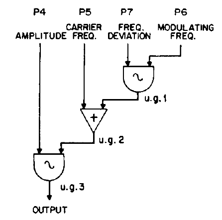
For one sinusoid modulating the frequency of a second,
frequency modulation can be written as:
\(f_c\) denotes the so called carrier frequency,
\(f_m\) the modulation frequency and \(I_m\)
the modulation index.
[Fig.1] shows a flow chart for this operation
in the style of MUSIC IV.
Flow chart for FM with two operators (Chowning, 1973).
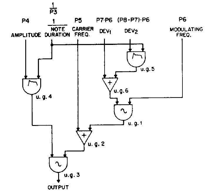
In many musical applications, the use of dynamic spectra is
desirable. The parameters of the above shown FM algorithm
are therefor controlled with temporal envelopes,
as shown in [Fig.2].
Especially the change of the modulation index over time
is important, since it results in percussive sound qualities.
In musical applications, multiple carriers and
modulators, referred to as operators,
are connected in different configurations, for
generating richer timbres.
Flow chart for dynamic FM with two operators (Chowning, 1973).
FM synthesis is considered an abstract algorithm.
It does not come with a related analysis approach
to generate desired sounds but they need to be
programmed or designed.
However, there are attempts towards an automatic
parametrization of FM synthesizers (Horner, 2003).
John Chowning, composer by profession, combined the novel
FM synthesis approach with digital spatialization techniques
to create quadraphonic pieces of electronic music
on a completely new level.
In Turenas, completed in 1972, artificial doppler shifts
and direct-to-reverberation techniques
are used to intensify the perceived motion
and distance of panned sounds
in the loudspeaker setup.
The sounds used in this piece are only generated by
means of FM, resulting in a characteristic quality
like the synthetic bell-like sounds beginning at 1:30
or the re-occuring short precussive events.
@article{chowning2011turenas,
    author = "Chowning, John",
    journal = "Proc. of the 17es Journées d’Informatique Musicale, Saint-Etienne, France",
    title = "{Turenas: the realization of a dream}",
    year = "2011"
}
@article{chowning1973thesynthesis,
    author = "Chowning, John M",
    journal = "Journal of the audio engineering society",
    number = "7",
    pages = "526–534",
    publisher = "Audio Engineering Society",
    title = "{The synthesis of complex audio spectra by means of frequency modulation}",
    volume = "21",
    year = "1973"
}
In some applications, like headless or embedded systems, it can be helpful to autostart the jack server, followed by additional programs for sound processing. In this way, a system can boot into the desired configuration without additional user interaction.
There are several ways of achieving this. The following example uses systemd services for a user named student.
The JACK Service
The JACK service needs to be started before the
clients. It is a system service and needs just a few
entries. This is a minimal example - depending on the application and hardware settings,
the arguments after ExecStart=/usr/bin/jackd need to be adjusted.
In order to start the service on every boot, it needs to be enabled:
$sudosystemctlenablejack.service
If desired, the service can also be deactivated:
$sudosystemctldisablejack.service
The Client Service(s)
Once the JACK service is enabled,
client software can be started.
A second service is created, which
is executed after the JACK service.
This is ensured by the additional
entries in the [Unit] section.
The example service launches a Puredata
patch without GUI:
The above content needs to be placed in the following file:
/etc/systemd/system/synth.service
The service can now be controlled with the above introduced
systemctl commands. When enabled, it starts on every boot
after the JACK server has been started:
Within the process function,
three oscillators are called in parallel by comma-separating them.
The :>_ operator collects their outputs, which are subsequently
devided by 3 and amplified.
Fourier Series in a Loop
The example fourier_series.dsp in the seminar's
Faust repository
makes use of the parallel directive within a loop,
allowing the use of more partials.
// fourier_series.dsp//// Generate a square wave through Fourier series.// - without control//// Henrik von Coler// 2020-05-06import("stdfaust.lib");// define a fundamental frequencyf0=100;// define the number of partialsn_partial=50;// partial function with one argument ()partial(partIDX)=(4/ma.PI)*os.oscrs(f)*volume// argumentswith{f=f0*(2*partIDX+1);volume=1/(2*partIDX+1);};// the processing function,// running 50 partials parallel// mono outputprocess=par(i,n_partial,partial(i)):>+;
The Faust Website Examples
The Faust website lists two examples for additive Synthesis.
Here, each partial is represented in the graphical
user interface with individual control for temporal
envelope parameters.
This allows playing a triggered sound with a
dynamic timbre.
Expressive Timbral Control
For using additive synthesis in an expressive way,
metaparameters are essential. It is desirable to control
the behavior of all partials and thus the timbre
with few meaningful controls.
Follow this link for a direct use in the Faust IDE:
The following example, found in the seminar's Faust repository, controlls the decrease in energy towards higher partials with a single parameter:
// exponential.dsp//// Additive synthesizer with controllable// exponential spectral decay.//// - continuous// - stereo output//// Henrik von Coler// 2022-10-26import("stdfaust.lib");gain=hslider("Master Gain",0,0,1,0.1):si.smoo;// define a fundamental frequencyf0=hslider("Pitch",50,10,1000,0.01):si.smoo;// define the number of partialsn_partial=200;slope=hslider("s",1,0.1,7,0.01):si.smoo;// partial functionpartial(partCNT,s)=os.oscrs(f)*volume// argumentswith{f=f0*(partCNT+1);volume=pow(s,0.5)*0.5*exp(s*-partCNT);};// the processing function,// running 200 partials parallel// summing them up and applying a global gainprocess=par(i,n_partial,partial(i,slope)):>_*gain<:_,_;
The sine wave can be considered the atomic unit of timbre and thus of musical sounds.
Additive synthesis and related approaches build musical sounds from scratch, using these integral components. When a sound is composed of several sinusoids, they are referred to as partials, regardless of their properties. Partials which are integer multiples of a fundamental frequency are called harmonics or overtones, when related to the first harmonic.
Fourier Series
According to the Fourier theorem, any periodic signal can be represented by an infinite sum of sinusoids with individual
amplitude \(a_i\)
frequency \(f_i\)
phase \(\varphi_i\)
\begin{equation*}
\displaystyle y = \sum\limits_{i=1}^{\infty} a_i \ sin(2 \pi f_i \ t +\varphi_i )
\end{equation*}
When applying this principle to musical sounds,
a simplified model can be used to generate basic timbres.
All sinusoidal components become integer multiples of
a fundamental frequency \(f_0\), so called harmonics,
with a maximum number of partials \(N_{part}\).
In an even further reduced model, the phases of the partials
can be ignored:
\begin{equation*}
\displaystyle y (t) = \sum\limits_{n=1}^{N_{part}} a_n(t) \ sin(2 \ \pi \ n \ f_0 (t) \ t)
\end{equation*}
As following sections on spectral modeling show, a more advanced model is needed
to synthesize musical sounds which are indistinguishable from the original.
This includes the partials' phase, inharmonicities as deviations from
exact integer multiples, noise components and transients.
However, depending of the number of partials and the
driving function for their parameters, this limited
formula can generate convincing harmonic sounds.
@article{di1998compositional,
    author = "Di Scipio, Agostino",
    title = "Compositional models in Xenakis's electroacoustic music",
    journal = "Perspectives of New Music",
    year = "1998",
    pages = "201--243",
    publisher = "JSTOR"
}
1870
Hermann von Helmholtz.
Die Lehre von den Tonempfindungen als physiologische Grundlage für die Theorie der Musik, 3. umgearbeitete Ausgabe.
Braunschweig: Vieweg, 1870. [details]
[BibTeX▼]
@book{vonhelmoltz1870dielehre,
    author = "von Helmholtz, Hermann",
    title = {Die Lehre von den Tonempfindungen als physiologische Grundlage f{\"u}r die Theorie der Musik, 3. umgearbeitete Ausgabe},
    publisher = "Braunschweig: Vieweg",
    year = "1870"
}
In the 1990s and early 2000s, most known
synthesis algorithms existed and provided
more and more convincing results, due to the
increasing computational power.
In order to overcome the drawbacks of individual
synthesis approaches, paradigms are combined
and novel, hybrid approaches are created.
Deep Learning & Neural Nets
Deep learning and neural nets have been used
as helper tools in sound synthesis for many years.
However, the direct use for the generation of
sound is rather new and currently the hot topic
in sound synthesis and processing.
Control and Mapping
Although the control of sound synthesis is not a
new topic, it remains one of the most active ones.
Synthesis algorithms are able to produce a large
variety of sounds in real-time since the 1990s,
but their integration into musical instruments
is a much wider topic, with many possibilities to explore
and stil lags behind.
While every digital sound synthesis approach
stands for itself due to its unique characteristics,
they all come with inherent
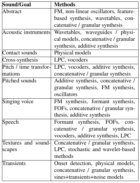
strengths and limitations with regard to specific tasks and applications.
[Fig.1] shows a list of synthesis goals with suitable
approaches by Misra et al. (2009).
In general, frequency-domain methods are less suited
for time-critical tasks, involving transients and
textures.
Also, the table in Fig.1 suggests the versatility of granular
and concatenative synthesis.
Synthesis goals and suitable approaches (Misra et al, 2009)
Many methods for sound synthesis - analog or digital -
have gained their status as an indipendent musical
instrument, with characteristic sound properties.
Some shaped the development of popular music and spawned new
musical genres.
This includes sampling - with a close link to rap music,
subractive synthesis in many ways and as backbone of
techno music, and FM synthesis - with the DX7
literally playing a part in most 1980s pop hits.
Such influential synthesizers have again been synthesized.
Virtual analog - also analog modeling - emulates vintage
subtractive synthesizers in hard- and software and
software synthesizers simulate classic FM synthesizers.
@article{chowning2011turenas,
    author = "Chowning, John",
    journal = "Proc. of the 17es Journées d’Informatique Musicale, Saint-Etienne, France",
    title = "{Turenas: the realization of a dream}",
    year = "2011"
}
@inproceedings{misra2009toward,
    author = "Misra, Ananya and Cook, Perry R",
    title = "{Toward Synthesized Environments: A Survey of Analysis and Synthesis Methods for Sound Designers and Composers}",
    booktitle = "Proceedings of the International Computer Music Conference (ICMC 2009)",
    year = "2009",
    location = "Montreal, Canada"
}
@inproceedings{smith2005viewpoints,
    author = "Smith, Julius O.",
    title = "{Viewpoints on the History of Digital Synthesis}",
    booktitle = "{ Proceedings of the International Computer Music Conference}",
    year = "1991",
    pages = "1–10"
}
1988
Miller S. Puckette.
The patcher.
In Proceedings of the International Computer Music Conference (ICMC). 1988. [details]
[BibTeX▼]
@inproceedings{puckette1988patcher,
    author = "Puckette, Miller S.",
    title = "The Patcher",
    booktitle = "{Proceedings of the International Computer Music Conference (ICMC)}",
    year = "1988",
    location = "Cologne, Germany"
}
@inproceedings{favreau1986software,
    author = "Favreau, Emmanuel and Fingerhut, Michel and Koechlin, Olivier and Potacsek, Patrick and Puckette, Miller S. and Rowe, Robert",
    title = "Software Developments for the 4X Real-Time System",
    booktitle = "{Proceedings of the International Computer Music Conference (ICMC)}",
    year = "1986",
    location = "Den Haag, The Netherlands"
}
@article{roads1980interview,
    author = "Roads, Curtis and Mathews, Max",
    title = "Interview with max mathews",
    journal = "Computer Music Journal",
    year = "1980",
    volume = "4",
    number = "4",
    pages = "15--22",
    publisher = "JSTOR"
}
1969
Max V. Mathews.
The Technology of Computer Music.
MIT Press, 1969. [details]
[BibTeX▼]
@book{mathews1969,
    author = "Mathews, Max V.",
    title = "{The Technology of Computer Music}",
    publisher = "MIT Press",
    year = "1969"
}
@article{mathews1963digital,
    author = "Mathews, Max V",
    title = "{The Digital Computer as a Musical Instrument}",
    journal = "Science",
    year = "1963",
    volume = "142",
    number = "3592",
    pages = "553--557",
    publisher = "JSTOR"
}
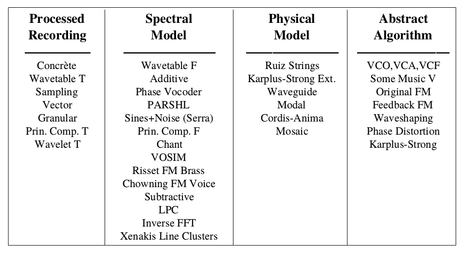
Digital methods for sound synthesis can be grouped
according to their underlying principle of operation.
In 1991, Smith proposed four basic categories,
shown in [Fig.2].
Already a technique in the analog domain,
more precisely in Musique Concrète,
this family of synthesis approaches makes
direct use of previously recorded sound for synthesis.
This can be the playback of complete sounds or the
extraction of short segments, such as grains or
a single period of a sound.
Spectral Models
Spectral models use mathmatical means for expressing
the spectra of sounds and their devopment over time.
They are usually receiver-based, since they model
the sound as it is heard, not as it is produced.
This paradigm already existed in the mechanical
world, as used by Hermann von Helmholtz in the
19th century and is based on even older signal models.
Physical Models
Physical Models are based on virtual acoustical
and mechanical units, realized through buffers
and LTI systems. Oscillators, resonating bodies
and acoustic conductors are thus combined as in
the mechanical domain.
Physical modeling is regarded a source-based
approach, since it deals with the actual
sound production.
Abstract Algorithm
If it is not processed sound, a spectral model
or a physical model, it is an abstract algorithm.
Algorithms from this category transfer methods
from other domains, like message transmission,
to the musical domain.
Missing Recent Approaches
Although a few categorisations could be debated,
the above introduced taxonomy is still valid
but misses some recent developments.
Methods based on neural networks and deep
learning for sound generation may be
considered a fifth taxon.
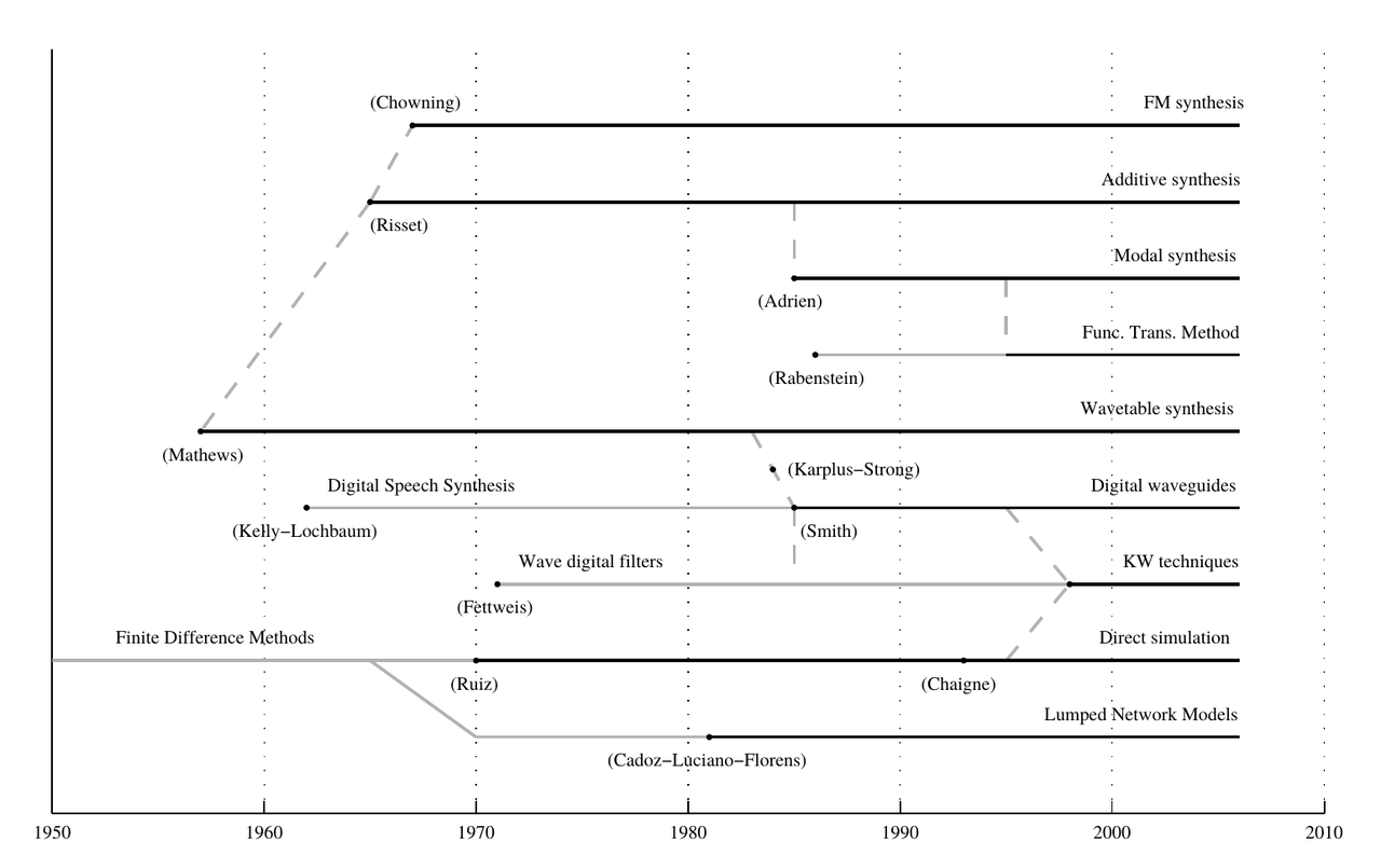
Family Tree
The synthesis experiments at Bell Labs are the
origin of most methods for digital sound synthesis.
[Fig.1] illustrates the relations for a subset of
synthesis approaches, starting with Mathews.
The foundation for many further developments was
laid when John Chowning brought the software MUSIC VI
to Stanford from a visit at Bell Labs (Chowning, 2011).
After migrating it to a PDP-6 computer,
Chowning worked on his groundbreaking digital compositions,
using the FM method and spatial techniques.
@article{chowning2011turenas,
    author = "Chowning, John",
    journal = "Proc. of the 17es Journées d’Informatique Musicale, Saint-Etienne, France",
    title = "{Turenas: the realization of a dream}",
    year = "2011"
}
@inproceedings{misra2009toward,
    author = "Misra, Ananya and Cook, Perry R",
    title = "{Toward Synthesized Environments: A Survey of Analysis and Synthesis Methods for Sound Designers and Composers}",
    booktitle = "Proceedings of the International Computer Music Conference (ICMC 2009)",
    year = "2009",
    location = "Montreal, Canada"
}
@inproceedings{smith2005viewpoints,
    author = "Smith, Julius O.",
    title = "{Viewpoints on the History of Digital Synthesis}",
    booktitle = "{ Proceedings of the International Computer Music Conference}",
    year = "1991",
    pages = "1–10"
}
1988
Miller S. Puckette.
The patcher.
In Proceedings of the International Computer Music Conference (ICMC). 1988. [details]
[BibTeX▼]
@inproceedings{puckette1988patcher,
    author = "Puckette, Miller S.",
    title = "The Patcher",
    booktitle = "{Proceedings of the International Computer Music Conference (ICMC)}",
    year = "1988",
    location = "Cologne, Germany"
}
@inproceedings{favreau1986software,
    author = "Favreau, Emmanuel and Fingerhut, Michel and Koechlin, Olivier and Potacsek, Patrick and Puckette, Miller S. and Rowe, Robert",
    title = "Software Developments for the 4X Real-Time System",
    booktitle = "{Proceedings of the International Computer Music Conference (ICMC)}",
    year = "1986",
    location = "Den Haag, The Netherlands"
}
@article{roads1980interview,
    author = "Roads, Curtis and Mathews, Max",
    title = "Interview with max mathews",
    journal = "Computer Music Journal",
    year = "1980",
    volume = "4",
    number = "4",
    pages = "15--22",
    publisher = "JSTOR"
}
1969
Max V. Mathews.
The Technology of Computer Music.
MIT Press, 1969. [details]
[BibTeX▼]
@book{mathews1969,
    author = "Mathews, Max V.",
    title = "{The Technology of Computer Music}",
    publisher = "MIT Press",
    year = "1969"
}
@article{mathews1963digital,
    author = "Mathews, Max V",
    title = "{The Digital Computer as a Musical Instrument}",
    journal = "Science",
    year = "1963",
    volume = "142",
    number = "3592",
    pages = "553--557",
    publisher = "JSTOR"
}
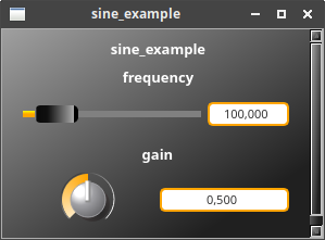
In Faust, control parameters are always declared with a graphic user interface element.
For some targets, these elements are ignored. For GUI targets, however, they are automatically
included in the final software. With the native Faust GUI, as used in standalone applications,
an example with two parameters may look like this:
This example implements a sine wave generator with controllable frequency and amplitude.
The following image shows the top level flow chart generated by Faust:
The frequency of the oscillator is controlled with a horizontal slider, whereas the element for controlling the gain is in knob style. Additional parameters (see the Faust documentation for details) define parameter ranges, initial value more.
import("stdfaust.lib");// input parameters with GUI elementsfreq=hslider("frequency",100,10,1000,0.001);gain=hslider("gain[style:knob]",0,0,1,0.001);// a sine oscillator with controllable frequency and amplitude:process=os.osc(freq)*gain;
The class makes use of Jupyter Notebooks for illustrating details of synthesis algorithms and their components.
Jupyter files for the class are organized in a Git Repository.
Use your own Jupyterlab or Jupyternotebook Instance
You can install your own of instance of JupyterLab or JupyterNotebook,
alongside the necessary libraries and use the examples from the
repository.
The repository can be used with an on line service like Binder.
Simply past the url of the repository to build a Docker image. This can take some time.
This link is a fast forward to the Binder of this repository: Quick Link