About

Puredate (PD) is the free and open source version of Max/MSP, also developed and maintained by Miller Puckette. PD is one of the best options for people new to computer music, due to the obvious signal flow. It is a very helpful for exploring the basics of sound synthesis and programming but can also be used for advanced applications: https://puredata.info/community/member-downloads/patches.

As a graphical programming environment, PD offers simple and flexible means for creating control and GUI software. There are a lot of great tutorials and examples online. This one features almost anything to know: http://write.flossmanuals.net/pure-data/

Working with PD Files

PD patches are organized in files with the .pd extension. This first patch is the well known Hello World! example, not using any audio processing:

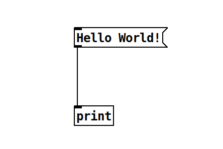
It introduces two concepts:

• A message, containing the string Hello World!.

• An object, namely print, printing the string to the PD console in the main window.

#N canvas 899 583 450 300 12;
#X obj 75 107 print;
#X msg 75 29 Hello World!;
#X connect 1 0 0 0;

References

Recordings

The corpus of speech was gathered in two group sessions, each with five persons, in the anechoic chamber at TU Berlin. For each speaker, the recording was annotated into regions of different valence and arousal and then segmented into syllables, automatically.

Features

Synthesis

The following example synthesizes a crowd with a valence of -90 and an arousal of 80, which can be categorized as frustrated, annoyed or upset. No virtual acoustic environment is used, and the result is rather direct:

References

References

Early Analog

John Cage's Williams Mix, realized in 1952-53 shows some of the earliest granular approaches.

Iannis Xenakis was the first to refer to Dennis Gabor's quantum theory and the elementary signal (Gabor, 1946) for musical applications.

Early Digital

The possibilities to use granular synthesis grew rapidly with the advent of digital sampling and new composers made use of the technique.

Barry Truax, who was visiting the TU Studio as guest professor in 2015-16 is known as one of the pioneers of digital granular composition (Truax, 1987). His soundscape-influenced works use the technique for generating rich textures, as in Riverrun:

Horacio Vaggione made use of granular processing for his mixed music pieces. The original Scir - for bass flute and tape (which is granular processed bass flute) - has ben produced at the TU Studio in 1988:

In 2018, the TU Studio performed the piece with flutist Erik Drescher and made a binaural recording:

Using 'soundfile'

Under the hood, using sound files in Faust is based on libsndfile. This part of Faust is less documented and lacks full integration. The soundfile primitive, which is the basis for reading and playing audio files, is not yet managed in the Faust Web IDE and can not be used with all targets.

When using wav files in Faust, their content is combined with the generated binary when compiling. Files can thus not be read dynamically. Compiling with support for managing audio files is enabled with the -soundfile flag:

$ faust2jaqt -soundfile sample_trigger.dsp

Samples With a Trigger

The soundfiles.lib library includes convinient functions for handling sound files and playing them:

https://github.com/grame-cncm/faustlibraries/blob/master/soundfiles.lib

Using the provided methods, basic use of audio files is granted with little code. The example sample_trigger.dsp makes use of the play method for soundfiles. A set of audio files is read and selected files can be triggered with buttons.

// sample_trigger.dsp
//
// Read files and make them playable with a trigger.
//
// - makes use of the
//
// Henrik von Coler
// 2020-05-28

import("stdfaust.lib");

// read a set of wav files
s = soundfile("label[url:{'../WAV/kick.wav'; '../WAV/cowbell.wav'; '../WAV/my_model.wav'}]", 1);

// a slider for controlling the level of all samples:
level = hslider("level",1,0,2,0.01);

// sample objects
kick = so.sound(s, 0);
bell = so.sound(s, 1);

process = kick.play( level, button("kick") ),  bell.play( level, button("bell")) :>  _   <: _,_ ;

Looping a Sample

sample_looper.dsp defines a looping function which can play a chosen sample with fracional playrates, allowing reverse looping.

// sample_looper.dsp
//
// Read a set of samples from wav files
//
// - loop sample with slider for speed
// - select active sample
//
// Henrik von Coler
// 2020-05-28

import("stdfaust.lib");

// read a set of wav files
s = soundfile("label[url:{'../WAV/kick.wav'; '../WAV/cowbell.wav'; '../WAV/my_model.wav'}]", 1);

// a slider for selecting a sound file:
file_idx = hslider("file_idx",0,0,2,1);

// a slider for controlling the playback speed:
speed = hslider("speed",1,-100,100,0.01);

// a logic for reverse loops (wrap to positive indices)
wrap(l,x) = select2((x>=0),l-abs(x),x);


// the loop function
loop(s, idx) = (idx, reader(s)) : outs(s)
with {

// get recent file's properties
length(s) = idx,0 : s : _,si.block(outputs(s)-1);
srate(s)  = idx,0 : s : !,_,si.block(outputs(s)-2);

// the playback position (a recursive counter)
reader(s) = (speed * float(srate(s)))/ma.SR : (+,length(s):fmod)~  _ : wrap(length(s)) : int;

// read from sample
outs(s)   = s : si.block(2), si.bus(outputs(s)-2);

};

process = loop(s,file_idx) <: _,_ ;

First Compositions & Musique Concrète

Halim El-Dabh was probably the first person to compose musical works with previously recorded material. His tape piece The Expression of Zaar dates back to 1944 and was realized in Cairo, Egypt. Only slightly later, after World War II, Pierre Schaeffer started his experiments with turntables. He recorded environmental sounds and musical instruments, arranged them, altered the playback speed and used loops in what then became musique concrète. These techniques are well-known nowadays, but were a completely novel experience in th 1940s.

Although an engineer by profession, Pierre Schaeffer did not only explore the technical means for composing with recorded sound. With the theory of the objet sonore he also lay the foundation for the theory of acousmatic music (Schaeffer, 2012).

The Cinq Études de bruits (1948), the first published works of musique concrète, use various sources and techniques.

After the first experiments, Schaeffer started to involve musicians for taking the concept to the next level. With Pierre Henry he realized the Symphonie pour un homme seul in 1950. This acousmatic composition made use of various additional techniques, including spatial aspects.

Early Popular Music

Experimental approaches in popular music took up the idea of sampling and integrated recorded sounds, using them especially for intro and outro effects. Since their pioneering 1967 album Sgt. Pepper’s Lonely Hearts Club Band, the Beatles worked with sounds from mammals, birds and insects in almoast all of their albums (Brumm, 1012). Other examples for early experiments with sampled material are the The Beach Boys and Pink Floyd.

Digital Sampling

Early devices capable of digital sampling are the Fairlight CMI (1979) and the Synclavier II (1980). These expensive, bulky workstations were already used in various productions.

Linn Drum

The Linn Drum (1982) represents a milestone in digital sampling. Using 8 bit technique, it offers a fixed set of drum samples with a very recognisable sound. It can be found in most 1980s pop productions in the charts.

Akai MPC60 & E-mu SP-1200

These were the first affordable devices which allowed the use of custom samples. They are essential instruments for the development of Rap music. The workflow of these Desktop devices allowed the sampling of vinyl for a use in new rhythmic structures. Albums like It Takes a Nation of Millions to Hold Us Back (1988) by Public Enemy rely on this technique as the main sound source (Evans, 2010).

VCO-VCA-VCF

The first example for subtractive synthesis implements a virtual chain of VCO, VCF and VCA, as shown in the Faust diagram in [Fig.1].

Fig.1

Faust diagram for the VCO-VCA-VCF example.

The three modules are definied as individual functions, with paramters controlled by horizontal sliders. In the processing function, they are chained using the : operator.

A resonant low pass from the filters.lib - the Faust Filters library - is used.

// sawtooth-filter.dsp
//
// First steps with a VCO-VCA-VCF setup.
// The three modules are connected in series.
//
// No anti-aliasing!
//
// - steady sound
// - control over f0, cutoff, resonance, gain
//
// Henrik von Coler
// 2020-05-17

import("stdfaust.lib");

//////////////////////////////////////////////////////////////////////////
// Control Parameters
//////////////////////////////////////////////////////////////////////////

cutoff      = hslider("Cutoff", 100, 5, 6000, 0.001):si.smoo;
f0          = hslider("Pitch", 100, 5, 16000, 0.001):si.smoo;
q           = hslider("Q", 1, 0.1, 5, 0.01):si.smoo;
gain        = hslider("Gain", 1, 0, 1, 0.01):si.smoo;

//////////////////////////////////////////////////////////////////////////
// Define three 'module' functions
//////////////////////////////////////////////////////////////////////////

vco        = os.sawtooth(f0);
vcf         = fi.resonlp(cutoff,q,1) ;
vca(x)    = gain * x;

//////////////////////////////////////////////////////////////////////////
// Define three 'modules'
//////////////////////////////////////////////////////////////////////////

voice =  vco  : vcf : vca;

process = voice  <: _,_ ;

Triggered

The example subtractive_triggered.dsp from the repository extends the previous sawtooth example with temporal envelopes for VCF and VCA and implements four voices with individual control. The block diagram is shown in [Fig.2].

Fig.2

Faust diagram for the triggered subtractive example.

• The example makes use of the Moog filter from the vaeffects.lib library of virtual analog filter effects.

• Individual control over the voices is realized through the % command within the voice() function.

// subtractive_triggered.dsp
//
// A four voice subtractive synth.
//
// - trigger
// - control over f0, cutoff, resonance, gain
//
// Henrik von Coler
// 2020-05-17

import("stdfaust.lib");

trigger0 =  button("trigger0 [midi:key 33]");
trigger1=  button("trigger1 [midi:key 34]");
trigger2=  button("trigger2 [midi:key 35]");
trigger3=  button("trigger3 [midi:key 36]");

//////////////////////////////////////////////////////////////////////////
// Define three 'module' functions
//////////////////////////////////////////////////////////////////////////

vco(f0)          = os.sawtooth(f0);
vcf(c,r)          = ve.moog_vcf(r,c);
vca(x,gain)    = gain * x;


//////////////////////////////////////////////////////////////////////////
// A function with envelopes
//////////////////////////////////////////////////////////////////////////

voice(index,trig) =  vco(f0) : vcf(fc,res) : vca(env1) * 0.5
with
{
// use an individual hslider for every
f0                = hslider("Pitch %index", 100, 5, 1000, 0.001):si.smoo;

//trig = button("trigger%index");

rel1 = hslider("rel_vca%index", 0.5, 0.01, 3, 0.01):si.smoo;
rel2 = hslider("rel_vcf%index", 0.25, 0.01, 3, 0.01):si.smoo;

env1 = en.arfe(0.02, rel1, 0,trig); // en.adsre(0.001,0.3,1,1,trig);
env2 = en.arfe(0.01, rel2, 0,trig); //en.adsre(0.001,0.3,1,1,trig);

cutoff = hslider("cutoff%index", 100, 5, 6000, 0.001):si.smoo;
res     = hslider("res%index", 0.1, 0, 1, 0.01):si.smoo;

fc         = 10+env2* cutoff;

};

process = voice(0,trigger0),voice(1,trigger1),voice(2,trigger2),voice(3,trigger3) :> _,_ ;

Ringmodulator with Audio Input

The Ringmodulator is a simple, characteristic audio effect which has been used in many contextes. There is a large variety of guitar effect pedals based on ringmodulation. Another popular application is alienating voices, as done in vintage SciFi movies. The following example ringmod-input.dsp from the Faust repository modulates an audio input signal with a sine wave of adjustable frequency.

// ringmod-input.dsp
//
// Ringmodulator for audio input
//
// - fader for controlling modulator frequency
// - fader for controlling mix of ringmod
//
// Henrik von Coler
// 2020-05-12

import("stdfaust.lib");

f_m     = hslider("Modulator Frequency",100,0.01,1000,0.1);

mix     = hslider("Modulation Mix",0.5,0,1,0.01);

am(x, fm) =  (1-mix) * x  +  mix * x *  os.osc(fm);

process(x) =     am(x,f_m) <: _,_;

AM - Ringmod Explorer

When used with both sinusoidal carrier and modulator, Ringmodulator an AM become precice means for generating timbres in electronic music contexts. The example am-ringmod.dsp makes the tonal difference between AM and Ringmodulation audible.

// am-ringmod.dsp
//
// Example for amplitude modulation
// and ringmodulation.
//
// - steady sound
// - adjustable frequencies
// - fader for morphing between am/ringmod
//
// Henrik von Coler
// 2020-05-11

import("stdfaust.lib");

f_x = hslider("Signal Frequency",100,0.01,1000,0.1);
f_m = hslider("Modulator Frequency",100,0.01,1000,0.1);

m_off = hslider("Modulator Offset",0,0,0.5,0.01);


am(fx, fm) = os.osc(fx) * ((1-m_off) * os.osc(fm) + m_off);


process =  am(f_x,f_m) <: _,_;

References

1997
• Miller S. Puckette. Pure Data. In Proceedings of the International Computer Music Conference (ICMC). Thessaloniki, \\ Greece, 1997.
[details] [BibTeX▼]
1988
• Miller S. Puckette. The patcher. In Proceedings of the International Computer Music Conference (ICMC). Computer Music Association, 1988.
Concatenative: Crowd Noise Synthesis
Two master's thesis in collaboration between Audiocommunication Group and IRCAM aimed at a parametric synthesis of crowd noises, more precisely of many people speaking simultaneously (Grimaldi, 2016; Knörzer, 2017). Using a concatenative approach, the resulting synthesis system can be used to dynamically change the affective state of the virtual crowd. The resulting algorithm was applied in user studies in virtual acoustic environments.
2017
• Grimaldi, Vincent and Böhm, Christoph and Weinzierl, Stefan and von Coler, Henrik. Parametric Synthesis of Crowd Noises in Virtual Acoustic Environments. In Proceedings of the 142nd Audio Engineering Society Convention. Audio Engineering Society, 2017.
• Christian Knörzer. Concatenative crowd noise synthesis. Master's thesis, TU Berlin, 2017.
2016
2006
• Diemo Schwarz. Concatenative sound synthesis: The early years. Journal of New Music Research, 35(1):3–22, 2006.
• Diemo Schwarz, Grégory Beller, Bruno Verbrugghe, and Sam Britton. Real-Time Corpus-Based Concatenative Synthesis with CataRT. In In DAFx. 2006.
2000
• Diemo Schwarz. A System for Data-Driven Concatenative Sound Synthesis. In Proceedings of the COST-G6 Conference on Digital Audio Effects (DAFx-00). Verona, Italy, 2000.
1989
• C. Hamon, E. Mouline, and F. Charpentier. A diphone synthesis system based on time-domain prosodic modifications of speech. In International Conference on Acoustics, Speech, and Signal Processing,, 238–241 vol.1. May 1989. doi:10.1109/ICASSP.1989.266409.
1986
• F. Charpentier and M. Stella. Diphone synthesis using an overlap-add technique for speech waveforms concatenation. In ICASSP '86. IEEE International Conference on Acoustics, Speech, and Signal Processing, volume 11, 2015–2018. April 1986. doi:10.1109/ICASSP.1986.1168657.
Concatenative: Introduction
Concatenative synthesis is an evolution of granular synthesis, first introduced in the context of speech synthesis and processing (Charpentier, 1986; Hamon, 1989).
Concatenative synthesis for musical applications has been introduced by Diemo Schwarz. Corpus-based concatenative synthesis (Schwarz, 2000; Schwarz 2006) splices audio recordings into units and calculates audio features for each unit. During synthesis, unit selection can be performed by navigating the multidimensional feature space and selected units are concatenated.
/images/Sound_Synthesis/concatenative/concatenative-flow-1.png
Fig.1
(Schwarz, 2006)
/images/Sound_Synthesis/concatenative/concatenative-flow-2.png
Fig.2
Granular: Faust Example
The grain_player.dsp example in the repository uses four parallel grain processes, as shown in [Fig.1].
/images/Sound_Synthesis/granular/grain_player.png
Four parallel grain players
The code below does not handle all problem cases. Depending on the sound material, changing the grain position may result in audible clicks. For high densities, grains are retriggered before their ampltude dacays to 0 - also resulting in clicks.
// grain_player.dsp
//
// Play a wave file in grains.
// - four grains
// - glitches when changing grain position
2004
• Curtis Roads. Microsound. The MIT Press, 2004. ISBN 0262681544.
1987
1946
• D. Gabor. Theory of communication. part 1: the analysis of information. Journal of the Institution of Electrical Engineers - Part III: Radio and Communication Engineering, 93(26):429–441, November 1946. doi:10.1049/ji-3-2.1946.0074.
Sampling: Using Audio Files in Faust
2012
• P. Schaeffer. In Search of a Concrete Music. Volume 15 of California Studies in 20th-Century Music. University of California Press, 2012. ISBN 9780520265745. Translated by C. North and J. Dack. URL: http://books.google.de/books?id=6nTruQAACAAJ.
• Henrik Brumm. Biomusic and popular culture: the use of animal sounds in the music of the beatles. Journal of Popular Music Studies, 24:25–38, 03 2012. doi:10.1111/j.1533-1598.2012.01314.x.
2010
Subtractive: Faust Examples