Waveshaping is one of the basic ways of distortion synthesis. In its simplest form it works like any overdrive effect by limiting a signal with a non-linear shaping function. Depending on the implementation, these shaping
functions can have any form.
The following example shows a simple tangential shaping function
$y=\mathrm{tanh}(g x)$. For high pre-gain values, the function converges towards a step function and the output of a sinusoidal imput signal becomes a square wave.
Faust is a functional audio programming
language, developed at GRAME, Lyon. It is a community-driven,
free open source project.
Faust is specifically suited for quickly designing
musical synthesis and processing software and
compiling it for a large variety of targets.
The fastest way for getting started with Faust
in the Faust online IDE which allows programming
and testing code in the browser, without any installation.
The online materials for the class Sound Synthesis- Building Instruments with Faust introduce the basics of the Faust language and give examples for different synthesis techniques.
Faust and Web Audio
Besides many targets, Faust can also be used to create ScriptProcessor nodes (Letz, 2015).
@inproceedings{letz2015faust,
    author = "Letz, Stephane and Denoux, Sarah and Orlarey, Yann and Fober, Dominique",
    title = "Faust audio DSP language in the Web",
    booktitle = "Proceedings of the Linux Audio Conference",
    year = "2015",
    location = "Mainz, Germany"
}
This first, simple Web Audio sonification application makes use
of the Weather API for real-time, browser-based sonification
of weather data.
For fetching data, a free subscription is necessary:
https://home.openweathermap.org
Once subscribed, the API key can be used to get current weather
information in the browser:
All entries of this data structure can be used as
synthesis parameters in a sonification system with
Web Audio.
Temperatures to Frequencies
Mapping
In this example we are using a simple frequency modulation
formula for turning temperature and humidity
into more or less pleasing (annoying) sounds.
The frequency of a first oscillator is derived
from the temperature:
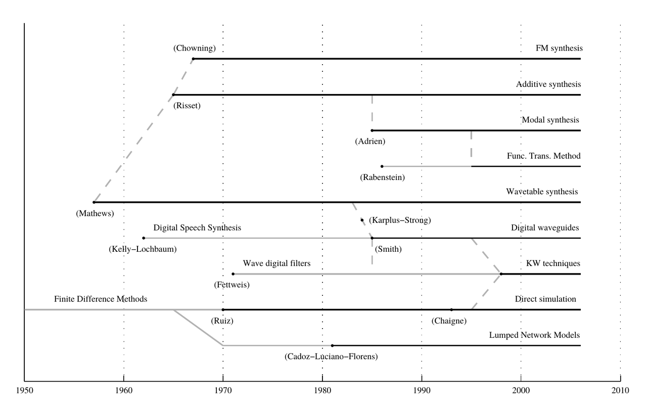
First experiments on digital sound creation took place 1951 in Australia, on the CSIRAC computer system.
Besides from these experiments, the development of digital sound synthesis dates back to the first experiments of Max Mathews at Bell Labs
in the mid 1950s. Mathews created the MUSIC I programming language for generating musical
sounds through synthesis of a single triangular waveform on an IBM 704.
The Silver Scale, realized by psychologist Newman Guttman in 1957, is one of the first ever digitally synthesized piece of music (Roads, 1980).
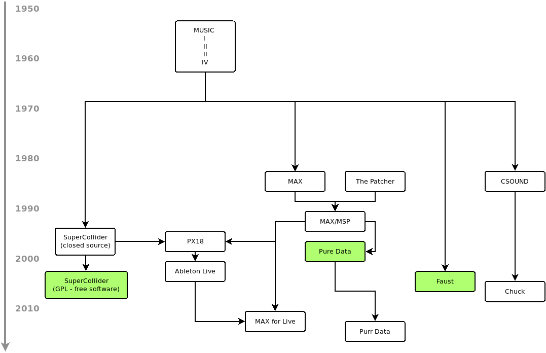
MUSIC and its versions (I, II, III, ...)
are direct or indirect ancestors to most
recent languages for sound processing.
Mathews defined the building blocks for digital sound synthesis and processing in these frameworks (Mathews, 1969, p. 48).
This concept of unit generators is still used today.
Although the first experiments sound amusing
from today's perspective, he already anticipated the
potential of the computer as a musical instrument:
“There are no theoretical limitations to the performance of the computer as a source of musical sounds, in contrast to the performance of ordinary instruments.” (Mathews, 1963)
Mathews created the first digital musical
pieces himself, but in order to fully explore the musical
potential, he was joined by composers, artists and other
researchers, such as Newman Guttman, James Tenney
and Jean Claude Risset.
Risset contributed to the development of electronic music
by exploring the possibilities of spectral analysis-resynthesis (1:20)
and psychoacoustic phenomena like the Shepard tone (4:43):
Later, the Bell Labs were visited
by many renowned composers of various styles genres, including
John Cage, Edgard Varèse and Laurie Spiegel (Park, 2009).
The work at Bell Labs will be in focus again in the
section on additive synthesis.
A Pedigree
The synthesis experiments at Bell Labs are the origin of most music programming languages and methods for digital sound synthesis.
On different branches, techniques developed from that seed (Bilbao, 2009):
The following family tree focuses on the tools used in this class and is thus without any claim to completeness:
Chowning & CCRMA
The foundation for many further developments was
laid when John Chowning brought the software MUSIC VI
to Stanford from a visit at Bell Labs in the 1060s.
After migrating it to a PDP-6 computer,
Chowning worked on his groundbreaking digital compositions,
such as Turenas (1972), using the frequency modulation synthesis (FM) and spatial techniques. Although in particular known for discovering the FM synthesis, these works are far more than mere studies of technical means:
Puckette & IRCAM
Most of the active music programming environments, such as Puredata, Max/MSP, SuperCollider or CSound, are descendants of the MUSIC languages. Graphical programming languages like Max/MSP
and Puredata were actually born as patching and mapping environments.
Their common ancestor, the Patcher (Puckette, 1986; Puckette, 1988), developed by Miller Puckette at IRCAM in the 1980s,
was a graphical environment for connecting MAX real-time processes and for controlling MIDI instruments.
The new means of programming and the increase in computational power allowed musique mixte with digital signal processing means. Pluton (1988-89) by Philippe Manoury is one of the first pieces to use MAX for processing piano sounds in real time (6:00-8:30):
@article{chowning2011turenas,
    author = "Chowning, John",
    journal = "Proc. of the 17es Journées d’Informatique Musicale, Saint-Etienne, France",
    title = "{Turenas: the realization of a dream}",
    year = "2011"
}
@inproceedings{misra2009toward,
    author = "Misra, Ananya and Cook, Perry R",
    title = "{Toward Synthesized Environments: A Survey of Analysis and Synthesis Methods for Sound Designers and Composers}",
    booktitle = "Proceedings of the International Computer Music Conference (ICMC 2009)",
    year = "2009",
    location = "Montreal, Canada"
}
@inproceedings{smith2005viewpoints,
    author = "Smith, Julius O.",
    title = "{Viewpoints on the History of Digital Synthesis}",
    booktitle = "{ Proceedings of the International Computer Music Conference}",
    year = "1991",
    pages = "1–10"
}
1988
Miller S. Puckette.
The patcher.
In Proceedings of the International Computer Music Conference (ICMC). 1988. [details]
[BibTeX▼]
@inproceedings{puckette1988patcher,
    author = "Puckette, Miller S.",
    title = "The Patcher",
    booktitle = "{Proceedings of the International Computer Music Conference (ICMC)}",
    year = "1988",
    location = "Cologne, Germany"
}
@inproceedings{favreau1986software,
    author = "Favreau, Emmanuel and Fingerhut, Michel and Koechlin, Olivier and Potacsek, Patrick and Puckette, Miller S. and Rowe, Robert",
    title = "Software Developments for the 4X Real-Time System",
    booktitle = "{Proceedings of the International Computer Music Conference (ICMC)}",
    year = "1986",
    location = "Den Haag, The Netherlands"
}
@article{roads1980interview,
    author = "Roads, Curtis and Mathews, Max",
    title = "Interview with max mathews",
    journal = "Computer Music Journal",
    year = "1980",
    volume = "4",
    number = "4",
    pages = "15--22",
    publisher = "JSTOR"
}
1969
Max V. Mathews.
The Technology of Computer Music.
MIT Press, 1969. [details]
[BibTeX▼]
@book{mathews1969,
    author = "Mathews, Max V.",
    title = "{The Technology of Computer Music}",
    publisher = "MIT Press",
    year = "1969"
}
@article{mathews1963digital,
    author = "Mathews, Max V",
    title = "{The Digital Computer as a Musical Instrument}",
    journal = "Science",
    year = "1963",
    volume = "142",
    number = "3592",
    pages = "553--557",
    publisher = "JSTOR"
}
SynthDefs are templates for Synths, which are
sent to a server:
// define a SynthDef and send it to the server(SynthDef(\sine_example,{// define arguments of the SynthDef|f=100,a=1|// calculate a sine wave with frequency and amplitudevarx=a*SinOsc.ar(f);// send the signal to the output bus '0'Out.ar(0,x);}).send(s);)
Create a Synth from a SynthDef
Once a SynthDef has been sent to the server,
instances can be created:
// create a synth from the SynthDef~my_synth=Synth(\sine_example,[\f,1000,\a,1]);// create another synth from the SynthDef~another_synth=Synth(\sine_example,[\f,1100,\a,1]);
Changing Synth Parameters
All parameters defined in the SynthDef of running synths can be changed,
using the associated variable on the client side:
// set a parameter~my_synth.set(\f,900);
Removing Synths
Running synths with a client-side
variable can be removed from the server:
// free the nodes~my_synth.free();~another_synth.free();
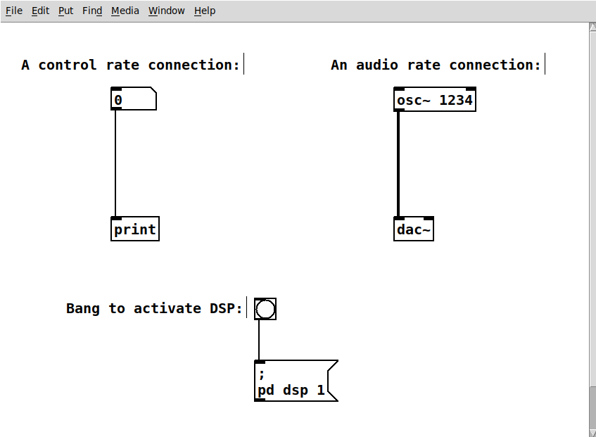
Like many other audio programming environments, PD makes a difference between control signals and audio signals. They run at different rates and can not be combined, unless converted. Audio operations require the DSP to be activated, whereas control rate signal work at any time. Objects define whether an outlet gets or outputs control or audio rate signals. Objects with audio inputs or outputs are usually named with a ~. Control rate connections are thinner than audio rate signals.
The example rates.pd simply shows
an audio and a control rate connection, with audio connections being thicker:
The example also introduces the osc~ oject, which generates a sine wave at 1234 Hz.
The message on the bottom of the patch is a patch-based way of activating the DSP, which can be very
helpful when working with automated and background processes.
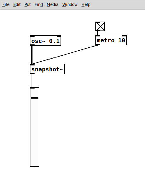
Audio to Control
Converting audio signals to control rate signals can be achieved with the snapshot~ object,
as done in the example audio-to-control.pd. A possible application is an envelope follower.
This object needs to be triggered to grab a snapshot, which is done with a metro object at 100 Hz in this example.
The output is a level indicator for the LFO at 0.1 Hz:
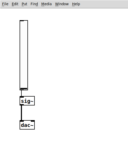
Control to Audio
Usually, control signals can be connected to audio inlets.
The conversion shown in the example audio-to-control.pd is thus less frequent.
However, in some cases it might be necessary to convert control signals to audio rate. This is done with the sig~ object:
The class Sound Synthesis
at TU Berlin makes use of the Raspberry PI as a development and runtime system for sound synthesis in C++ (von Coler, 2017).
Firtly, this is the cheapest way of setting up a computer pool with unified hard- and software.
In addition, the PIs can serve as standalone synthesizers and sonification tools.
All examples can be found in a dedicated software repository.
The full development system is based on free,
open source software.
The examples are based on the JACK API for audio input and output,
RtAudio for MIDI,
as well as the liblo for OSC communication and libyaml-cpp
for data and configuration files.
The advantage and disadvantage of this setup is that every element needs
to be implemented from scratch. In this way, synthesis algorithms can be
understood in detail and customized without limitations.
For quick solutions it makes sense to switch to a framework
with more basic elements.
The source code can also be used on any Linux system,
provided the necessary libraries are installed.
@inproceedings{voncoler2017teaching,
    author = "von Coler, Henrik and Runge, David",
    title = "Teaching Sound Synthesis in C/C++ on the Raspberry Pi",
    booktitle = "Proceedings of the Linux Audio Conference",
    year = "2017",
    location = "Saint-Etienne, France"
}
The Karplus-Strong algorithm is not exactly a physical model, but it can be considered a preliminary stage to waveguides. The algorithm is based on a ringbuffer, filled with (white) noise, which is then manipulated. With very simple means, Karplus-Strong can synthesize sounds with the characteristics of plucked strings. Although not entirely realistic, the result has a intriguing individual character.
Ringbuffers are the central element of the Karplus-Strong algorithm. As the name suggests, they are FIFO (first in - first out) buffers, with beginning and end connected.
A ringbuffer with N samples can be visualized as follows:
If a ringbuffer is filled with a sequence of white noise, it can be used for creating a white tone - a harmonic sound with a strong overtone structure.
Without resampling, the ring buffer can be shifted by one sample each $1/f_s$ seconds.
The resulting pitch of the sound is then determined by the buffer size:
$$f_0 = \frac{f_s}{N}$$
For a sampling rate of $48000$ Hz, a ringbuffer with a length of $N=200$ samples, results in the following pitch:
The spectrum of the white tone includes all harmonics up to the Nyquist frequency with a random amplitude. The overtone structure is individual for every white noise sequence, as is the timbre. These are three versions, started with an individual noise sequence of $N=400$ samples.
Karplus-Strong makes use of the random buffer and combines it with a moving average filter.
In the most basic form, two samples are read from the buffer $b$, starting from index $i$ (the playhead), and the average of both samples is written to the buffer. An additional gain factor - set to $0.95$ in this example, results in a faster decay:
$$ b[i] = 0.5 (b[i] + b[i+1])$$
$b[i]$ is directly sent to the output $y$ in each step:
$$y[i] = b[i]$$
$i$ is increased, until it reaches $N$ and continues from the beginning. The following image shows this for $i=3$:
The result of this circular smoothing is a gradual decrease in high frequencies. The sound begins with a metallic transient:
A faster decay of high frequencies can be achieved by larger moving average filters. This example uses a moving average of $10$ samples and a gain of $0.95$.
During the past decades, the subtractive principle has been implemented in many different ways, evolving along with the technology. Although based on the same principle, different families of subtractive synthesizers can be identified, all based on the same basic components. Representatives of these families have different characteristics and are used for different musical applications. Without claim to completeness these families are:
Analog modular
Analog monophonic
Analog polyphonic
Virtual analog / analog modeling
Analog Modular
The first subtractive synthesizers were large, cupboard-like devices and rather expensive. Although multiple voices are possible, they were designed as monophonic instruments. Two well known and opposite examples are the first models released by Bob Moog on the US east coast and Don Buchla on the west coast. The latter makes use of distortion techniques, whereas the Moog systems used the standard subtractive paradigm.
Moog Synthesizer (1965)
Switched on Bach, Wendy Carlos, 1968
Bob Moog brought the typical VCO-VCA-VCF approach in a rack with a keyboard.
It could hence be performed like a typical piano-like instrument.
In productions like Switched on Bach it was made polyphonic through dubbing with tape recording techniques.
This video shows the artist, Wendy Carlos, in an interview (since the LP is not available there):
Analog Monophonic
Analog monophonic synthesizers used the same techniques,
yet in a more compact design and not fully modular.
This made them more affordable and hence more
disseminated and used.
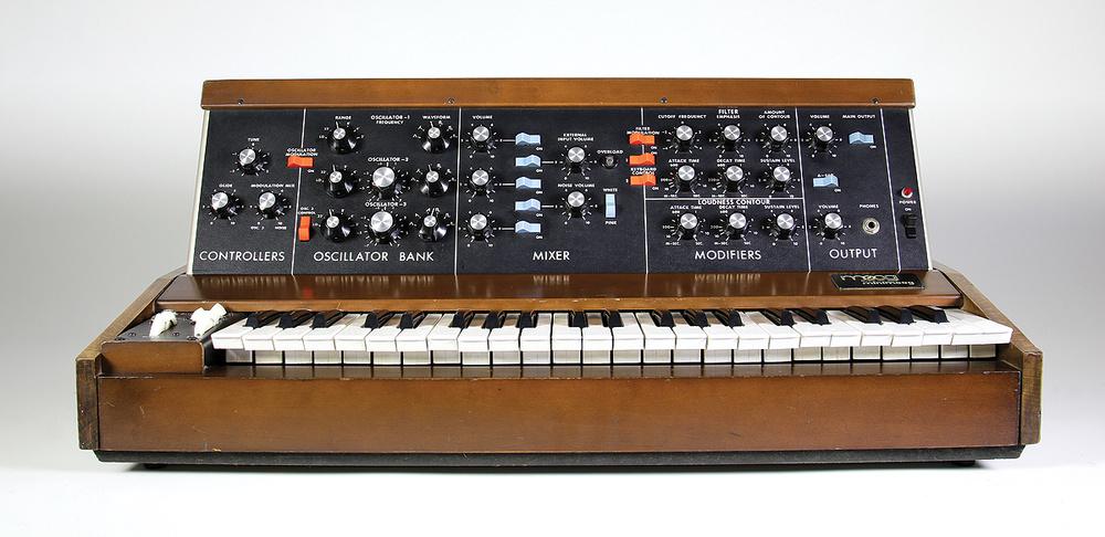
Minimoog Model D (1970)
The idea of monophonic analog subtractive synthesis - and maybe of the synthesizer in general -
is usually associated with the Minimoog.
Designed as a fully integrated musical instrument, the Minimoog could be used
in virtuous expressive musical performances, was portable and affordable.
Chick Corea's Minimoog solo, starting at 4:20, is an example of a virtuous performance, making use of modwheel and pitchbend:
EMS VCS 3 (1969)
The semi-modular EMS allows access to the signal flow with a patching matrix.
It is thus especially suited for experimental sounds, as used by Pink Floyd in
Welcome to the Machine for the wobbling machine sounds in the beginning:
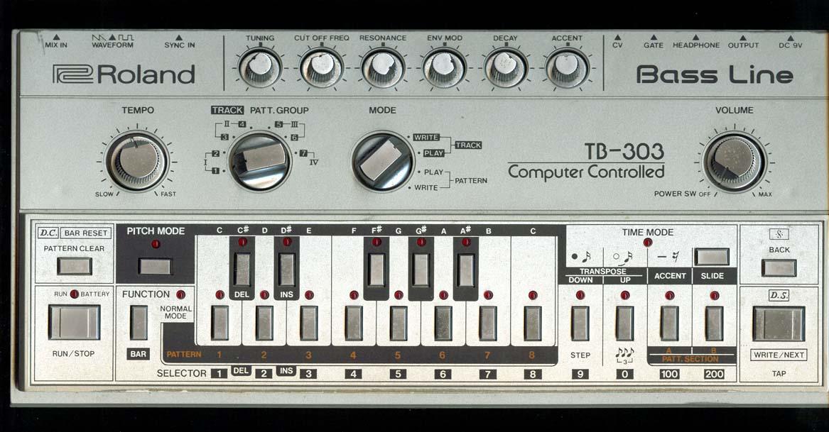
Roland TB 303 (1982)
Although released several years later - and for
a different application - the TB303 fits
best into this family.
The TB 303 was intended to be used as an
accompanying instrument for musicians.
It has a different interface, a programmable
step sequencer.
Due to the quirky filters it failed as a bass accompaniment but gave birth to techno and related genres.
It creates the typical acid basses and leads:
Analog Polyphonic
After the monophonic analog synths of the 70s, which were intended as solo instruments, came the polyphonic ones.
Polyphonic analog synthesizers shaped the sound of 80s pop (and especially synth-pop)
music with their recognizable sound, often used as pads and harmonic foundation or for bass lines.
Yamaha CS-80 (1977)
Oberheim OBx (1979)
Virtual Analog
When digital technology was ready, it took over
and various synthesizers were released which emulated
the principles of subtractive synthesis.
These devices were much cheaper and the digital
means could provide more voices with better memory options.
Virtual analog synthesizers were the backbone of
trance development. They lack some of the analog warmth but are tighter in sound. Some examples: