Like the sawtooth, the square wave shows the occurrence of ripples at the steep edges of the waveform. The higher the number of partials, the denser the ripples. This is referred to as the Gibbs phenomenon.
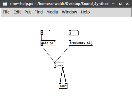
On linux systems this will create a file sine~.pd_linux,
on MacOS a file sine~.pd_darwin. Place the file in
your PD search paths and use it, as in the help file
sine~-help.pd. Parameters are set with messages.
Parallel processes in Faust are separated with the , operator.
The following example uses two square wave oscillators, each passing through
a lowpass filter. These chains are running in parallel, creating an output signal
with two channels for the left and right audio output:
This example is a parallel combination of two sequential compositions.
In Faust syntax, these need to be put in parenthesis.
The Faust project features a rich set of properly documented examples. Nevertheless, this class has an accompanying Git Repository for code snippets and small tutorials.
Links
There are a couple of links, which reappear as references in this lecture or can be used as additional resources.
@inproceedings{michon2018faust,
    author = "Michon, Romain and Smith, Julius and Chafe, Chris and Wang, Ge and Wright, Matthew",
    title = "The faust physical modeling library: a modular playground for the digital luthier",
    booktitle = "International Faust Conference",
    year = "2018"
}
The IEM Plug-in Suite was created by staff and students student of the Institute of Electronic Music and Acoustics in Graz. It is free and open source. Downloads and documentation can be found here https://plugins.iem.at/.
An in depth documentation of the IEM plugins features detailed information on installing and using the tools inside Reaper: https://plugins.iem.at/docs/.
The following pages include additional information on how to use the plugins with external software for control and processing, such as PD, SuperCollider and others.
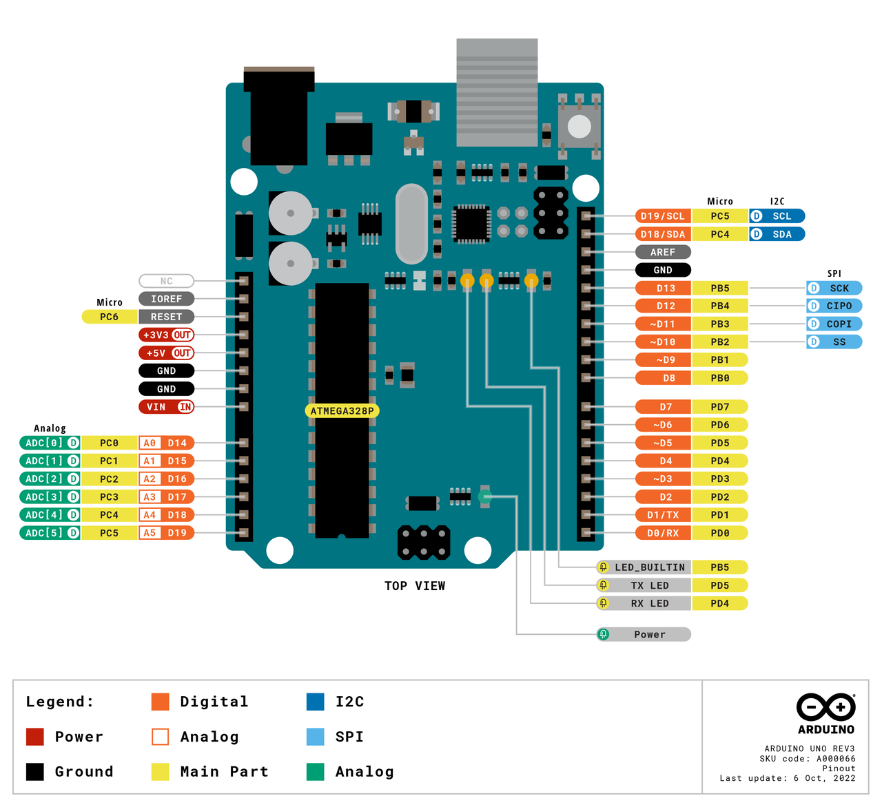
For all examples in this section, the Arduino UNO is used.
The documentation on the official Arduino website
covers all details on the connection possibilities and many examples to get started.
The most important bit of information for most tutorials and basic
applications is the pinout map:
Besides power and ground pins, the following connections are of interest for these examples:
6 analog inputs (0-5V)
14 digital pins (in and output mode can be set for each pin)
5 PWM output pins
serial receive
serial transmit
The Sensor
This very first step shows how to use basic sensors with the Arduino. These sensors are variable resistors, which change their
conductivity based on physical quantities. Examples are temperature, distance or force.
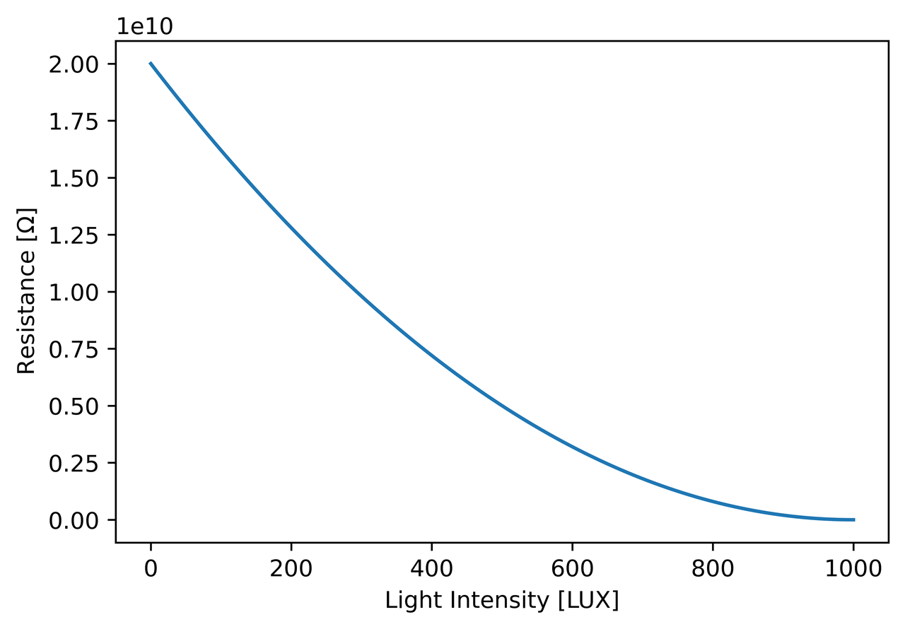
The following examples us a light dependent resistor (LDR). The brighter the light it is exposed to,
the lower its resistance.
Figure: Approximated curve of the LDR in this example.
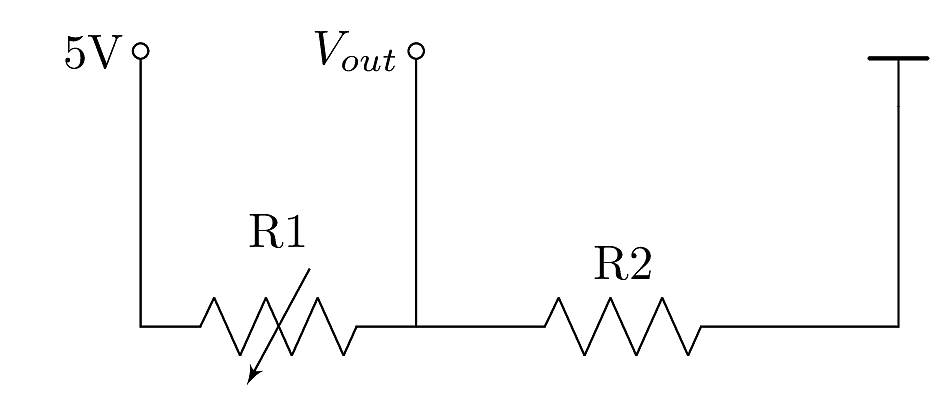
The Voltage Divider
In order to use the light dependent sensor in a measurement setup, a so called voltage divider is needed.
It compares the variable resistor R1 (in this case the LDR) with a fixed resistor R2:
Figure: Voltage divider circuit.
For a full use of the voltage range, R3 needs to be chosen properly.
The voltage measured at the output depends on the reference voltage of 5V and the ratio between the two resistors:
$$
V_{out} = 5V \frac{R_2}{R_1 + R_2}
$$
Some components, like potentiometers and faders, have the voltage divider integrated
and thus have three pins for connection.
They do not require an additional resistor.
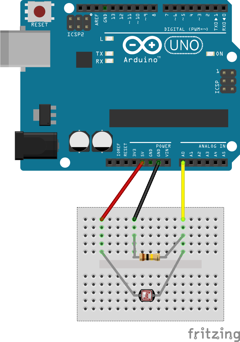
Breadboard Wiring
The above-shown circuit can be realized using all components, a mini breadboard and three jumper cables.
The documentation on the original Arduino website (Getting Started with Arduino
introduces the board with all its connection capabilities in detail.
For this example, we need a small breadboard, the LDR, one resistor and three jumper cables.
A $100 \Omega$ resistor is chosen.
For first steps, the Arduino can be powered via USB, which will also be used to read
the sensor data into the Arduino serial monitor.
Figure: Arduino breadboard wiring.
Arduino Code
The easiest way to program an Arduino is the dedicated Arduino IDE, which is available for all major operating systems.
Install and use instructions are thoroughly documented on the official Arduino website.
The Arduino code for testing this sensor circuit is minimalistic.
Like most Arduino sketches, basic setup is carried out in the setup() function on boot.
In this case, the serial interface is started with a baud rate (speed in symbols per second) of 9600 bauds.
Afterwards, the loop() function is carried out infinitely.
It reads the given voltage at the selected pin A0 and prints it to the serial output.
Follow the instructions on the Arduino website to upload the below code to your board. In general,
the serial port of the board needs to be selected in the IDE's dropdown manual,
alongside the Arduino model - in this case the Arduino UNO.
Without any manipulation, the values from the analogRead() function range from 0 to 1024,
since the Arduino analog-digital converters have 10 bit resolution:
Max for Live makes max patches run as part of an Ableton Live session.
Depending on the nature of the patch, it can be inserted as a device in Audio or MIDI tracks
by drag and drop.
MIDI and audio outlets of the patch will be visible and usable inside Live like the
connection of any other component.
Over the years, many devices have been created by the community, some for free, some for sale: https://maxforlive.com/
The concept and its details are best described on Ableton's Live page.
This short introduction should only cover the very basics for a quick start.
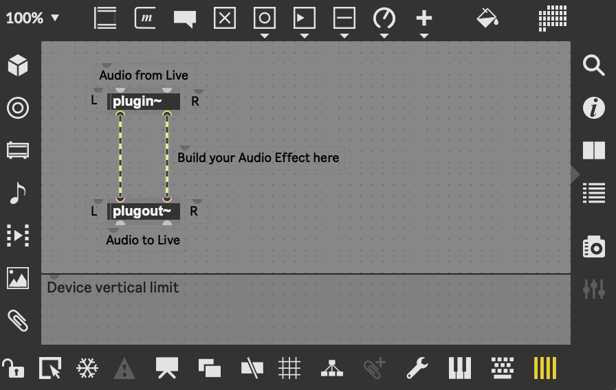
Max Audio Effects
Dragging the default Max Audio Effect into a track gives a basic patch
connecting audio inlets (plugin~) with audio outlets (plugout~).
Any processing can be inserted in between.
The default Max Audio Effect.
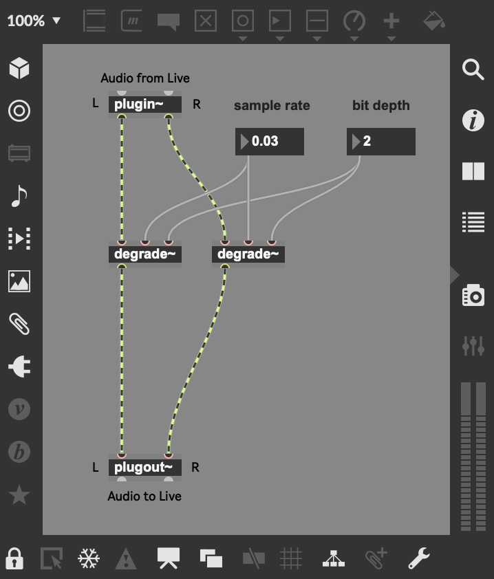
The following example uses the degrade~ object inside a Max Audio Effect.
A degrader effect inside Max for Live.
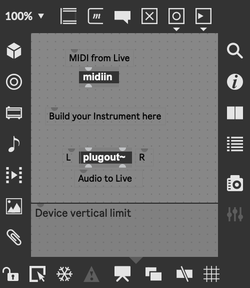
Max Instruments
The default Max Instrument can be dragged into a MIDI channel. It gives
a patch with a midiin object to receive any incoming MIDI data and
the plugout~ object to send audio into Live.
Unlike the default Audio Effect, this patch is not functional.
The default Max Instrument.
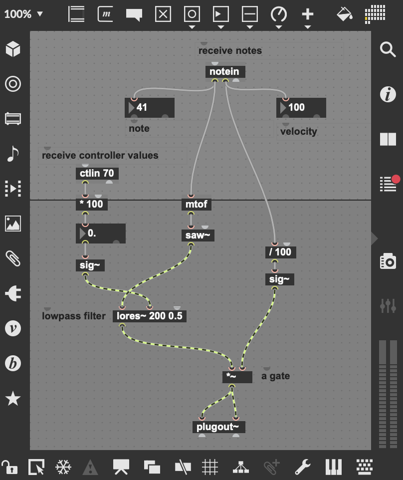
Like the midiin object, other MIDI objects in Max can also be used inside Max For Live devices.
The following mini saw example shows how to control a patch with MIDI from Live, using the notein
and the ctlin objects.
A mini saw synthesizer.
Automation to Max for Live
The Inspector View
Although controlling Max for Live with MIDI is a good solution for many applications,
Device Parameter Automation offers more flexibility and can also be used in audio channels.
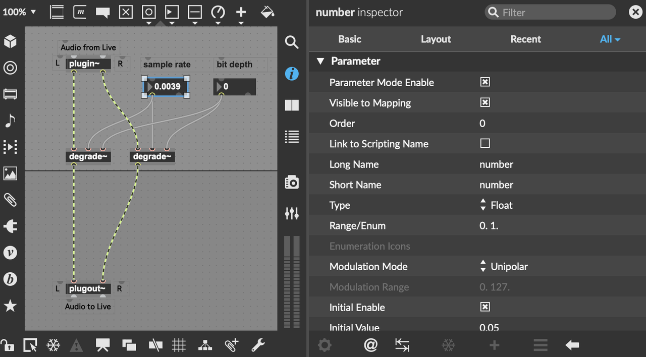
Most parameters in a Max for Live patch can be activated for automation, by editing inside the number inspector:
The number inspector in Max for Live.
The following adjustments need to be made:
Parameter Mode Enable: check
Name (long/short): foo
Type: match parameter
Range: match parameter
Modulation Mode: match parameter
Parameter Visibility: Automated and Stored
Track Automation
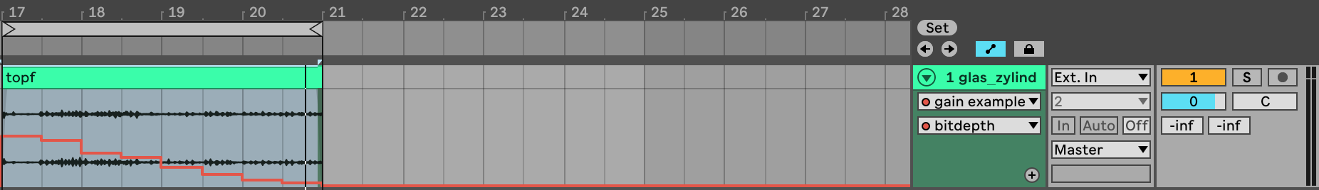
After making the Max for Live parameters ready for automation, the general automation mode needs to be
enabled in the Arranger view (the tiny blue button above the audio track).
Afterwards, each tack shows the available automation parameters and they can be edited.
Automation in the arranger window.
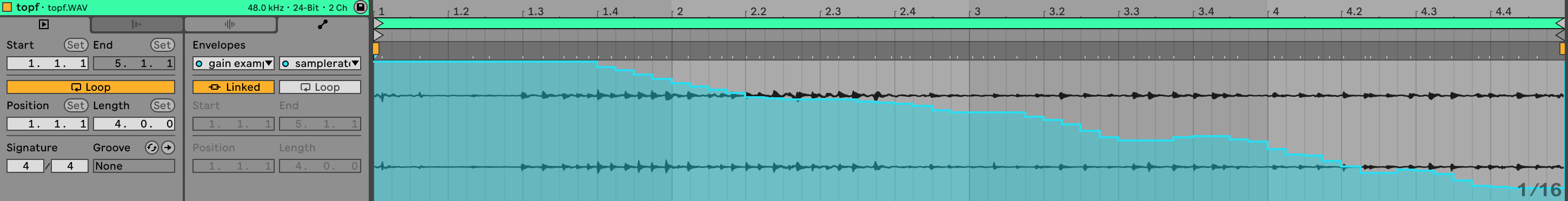
Clip Automation
The automation panel in the clip view gives access to all activated Max for Live parameters.
This kind of modulation is tightly linked to the audio material, which can be both helpful and complicated.
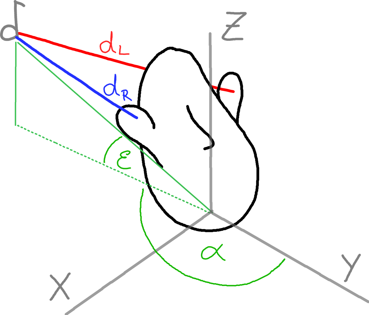
Two-ear (binaural) listening encodes information on the direction and distance
of a sound source by several cues. Figure 1 shows a listener with a sound source and its
properties azimuth elevation and distance.
Interaural cues are based on the signal of both ears,
more precisely their differences. They are in particular relevant for the horizontal Localization,
respectively the azimuth:
interaural time differences (medium frequencies)
interaural level differences (high frequencies)
interaural phase differences (low frequencies)
In addition to the interaural cues, the coloration gives information on the elevation of
a sound source, as well as on opposing azimuth angles which have identical interaural cues.
Figure 1: Sound source with angles and distances to left and right ear.
Binaural Recording Technology
Dummy Head
Dummy Head recordings use the principles of binaural listening with two microphones and a
model head, carrying these microphones at the position of the ear drum.
When the dummy head is placed in any environment, it listens and records the signals of both ears to two channels.
Many binaural records were released during the 1970s, yet without larger success.
With the increased use of in ear headphones and streaming, binaural techniques became more and more popular
in the 2010s. ASMR artists, for example, use close-up binaural recordings to create intimate
@article{wenzel1993localization,
    author = "Wenzel, Elizabeth M and Arruda, Marianne and Kistler, Doris J and Wightman, Frederic L",
    title = "Localization using nonindividualized head-related transfer functions",
    journal = "The Journal of the Acoustical Society of America",
    volume = "94",
    number = "1",
    pages = "111--123",
    year = "1993",
    publisher = "Acoustical Society of America"
}
By default Ansible logs into every machine via SSH. hosts: web tells ansible
to execute following tasks on all machines in the inventory group web.
Installing packages with APT requires superuser permissions. become: yes tells
Ansible to become root. The default method for this is sudo.
The biggest benefit over shell scripts is that it is possible to describe the
state of a machine. In the example four packages will be installed.
Only jackd2 will be updated if it is already present.
---
Inventory
For executing our new playbook Ansible needs to know what machines are in our
inventory. The inventory can be written in INI or YAML syntax.
[local]localhost[web]google.defacebook.de
The default location for your inventory file is /etc/ansible/hosts.
For more information for creating your inventory see the official
user guide.
---
ansible.cfg
A separate inventory file can be set for your project in an Ansible configuration
file ansible.cfg:
This file sets the location of your inventory file to ./hosts. Furthermore
the default SSH user as well as the sudo user gets set to studio.
---
Executing a Playbook
Executing our playbook file install_basic.yml:
ansible-playbook install_basic.yml -k -K
For this to work every machine in group web must have a user studio with the
same password. The flag -k lets Ansible ask for a SSH password. -K is for the
sudo password.
If there's a SSH key for user studio on all machines, no SSH password has
to be typed, but the password for sudo is still necessary.