
Flask
The Meson build system
Meson is a modern and fast build system with a lot of features. You can find its documentation at mesonbuild.com. Meson is written in Python. Meson has different backends (Ninja, VS*, Xcode, …).
Installing Meson and Ninja
The best maintained backend of Meson is Ninja. Installing both can be done with your distribution's package manager, with PIP, Homebrew, etc. The version for your user and your superuser has to be the same.
Fedora
Debian/Ubuntu
macOS:
PIP:
Build
Meson builds in a separate directory. It doesn't touch anything of your project. This way you can have seperate debug and release build directories for example.
Prepare your build directory:
meson builddir                                  # defaults to debug build

## Additional build directories
meson --buildtype release build_release         # release build
meson --buildtype debugoptimized build_debug    # optimized debug build
```
Now build with Ninja:
Install with:
Configuration
If you are in a build directory, meson configure shows you all available options.
Audio Input & Output in PD
All objects which have audio inputs or outputs are written with a tilde as last character of their name(~).
The two objects introduced in this minimal example get audio signals from the
audio interface (adc~ - for analog-digital-conversion),
respectively send them to the audio interface (dac~, for digital-analog-conversion):
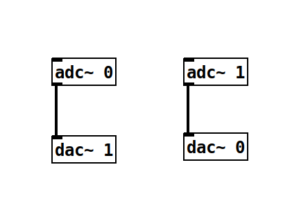
Both adc~ and dac~ have one creation argument - the index of the input our output, counting from 1.
The above shown example gets the left and the right channel from the audio hardware and swaps them,
before sending them to the audio output.
Activating DSP
PD patches will only process audio when DSP has been activated.
This can be done in the Media section of the top menu or with the shortcut Ctrl+/ (Cmd+/ on Mac).
DSP can always be killed using the shortcut Ctrl+. (Cmd+. on Mac).
References
1997
- Miller S. Puckette.
Pure Data.
In Proceedings of the International Computer Music Conference (ICMC). Thessaloniki, \\ Greece, 1997.
[details] [BibTeX▼]
1988
- Miller S. Puckette.
The patcher.
In Proceedings of the International Computer Music Conference (ICMC). Computer Music Association, 1988.
[details] [BibTeX▼]
Understanding Ambisonics Signals
Spherical Harmonics
Ambisonics is based on a decomposition of a sound field into spherical harmonics. These spherical harmonics encode the sound field according to different axes, respectively angles of incidence. The number of Ambisonics channels $N$ is equal to the number of spherical harmonics. It can be calculated for a given order $M$ with the following formula:
\begin{equation*}
N = (M+1)^2
\end{equation*}
Figure 1 shows the first 16 spherical harmonics. The first row ($N=1$) is the omnidirectional sound pressure for the order $M=0$. Rows 1-2 together represent the $N=4$ spherical harmonics of the first order Ambisonics signal, rows 1-3 correspond to $M=2$, respectively $N=9$ and rows 1-4 to the third order Ambisonics signal with $N=16$ spherical harmonics. First order ambisonics is sufficient to encode a threedimensional sound field. The higher the Ambisonics order, the more precise the directional encoding.
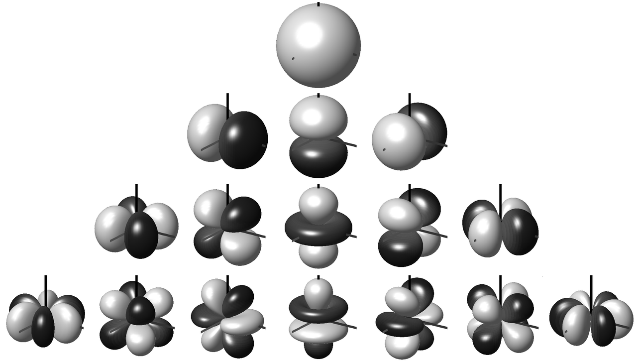
Fig. 1: Spherical harmonics up to order 3 [1].
Ambisonic Formats
An Ambisonics B Format file or signal carries all $N$ spherical harmonics. Figure 2 shows a first order B Format signal.
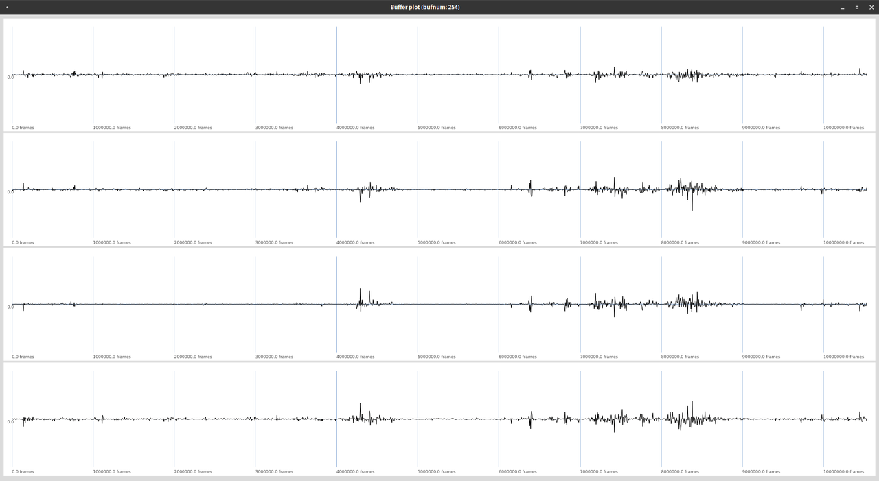
Fig. 2: Four channels of a first order Ambisonics signal.
There are different conventions for the sequence of the individual signals, as well as for the normalization.
References
2015
- Matthias Frank, Franz Zotter, and Alois Sontacchi.
Producing 3d audio in ambisonics.
In Audio Engineering Society Conference: 57th International Conference: The Future of Audio Entertainment Technology–Cinema, Television and the Internet. Audio Engineering Society, 2015.
[details] [BibTeX▼]
2009
- Frank Melchior, Andreas Gräfe, and Andreas Partzsch.
Spatial audio authoring for ambisonics reproduction.
In Proc. of the Ambisonics Symposium. 2009.
[details] [BibTeX▼]
Using Ambisonics Recordings
The following example uses a first order Ambisonics recording, and converts it to a binaural signal, using the SC-HOA tools. The file can be downloaded here:
http://ringbuffer.org/download/audio/210321_011_Raven.wav
The Recording
A Format
The file is a first order Ambisonics recording, shot outdoors with a Zoom H3-VR. The original raw material is the so called A Format. It features one channel for each microphone.
B Format
The file in the download is a first order Ambisonics B format recording. This is a standardized format, encoding the sound field in spherical harmonics.
Load HOA Stuff
Load Ambisonics File into Buffer
The following code works with the file located in the same directory as the working script. A buffer is used to read the four channel file:
Create a Playback Node
The buffer can be used with a PlayBuf UGen, to create a node which plays the
sample in a continuous loop.
An extra 4-channel audio bus is created for the Ambisonics signal.
It can be monitored to check whether the signal is playing properly:
Create Binaural Decoder
An second node is created for decoding the Ambisonics signal, allowing an additional rotation of the sound image. It has three arguments for setting pitch, roll and yaw. Make sure to move the new node after the playback node to get an audible result:
// create a decoder with angles as arguments:
(

~decoder = {

    arg pitch=0, roll=0, yaw=0;

    var input    = In.ar(~ambi_BUS.index, 4);

    var rotated  = HOATransRotateXYZ.ar(1, input, pitch, roll, yaw);

    var binaural = HOABinaural.ar(1,rotated);

    Out.ar(0, binaural);

}.play;

)

// move after playback node
~decoder.moveAfter(~playback);
Exercises
John Cage's Williams Mix
John Cage's Williams Mix (1952) is an early example of multichannel spatial audio. Cage used eight single track tape machines, without proper synchronization, which was not yet invented (Gurevich, 2015). In the time of tape editing, the first ever eight channel piece of music was realized with the assistance of Louis and Bebe Barron (recording), as well as Earle Brown, Morton Feldman, and David Tudor. A paper score of 193 pages gave instructions for the editing procedure:
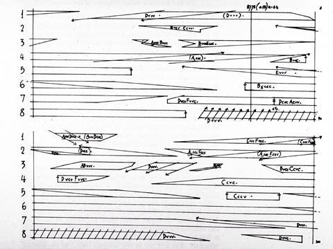
Splicing score for the Williams Mix.
Stereo Version
Although this stereo version does not capture the full spatial experience, it conveys the granular nature of the piece:
Spatial Sound Synthesis
Spectral Spatialization
Spectral spatialization is an advanced form of spatialization, which is based on a separation of audio signals into frequency bands (Kim-Boyle, 2008). These frequency bands can be distributed in space which allows a dynamic spreading of existing sound material. Spectral spatialization methods are found in many electroacoustic compositions and live electronic performances.
Spatial Sound Synthesis
Spatial sound synthesis refers to spatialization at an early stage in the synthesis process. In contrast to classic spatialization of existing sources, this results in spatially distributed sounds. Approaches towards spatial sound synthesis have been presented for most known synthesis principles, including additive synthesis (Topper, 2002), granular synthesis (Roads, 2004), physical modeling (Mueller, 2009) and modulation synthesis (McGee, 2015).
References
2017
-
Grimaldi, Vincent and Böhm, Christoph and Weinzierl, Stefan and von Coler, Henrik.
Parametric Synthesis of Crowd Noises in Virtual Acoustic Environments.
In Proceedings of the 142nd Audio Engineering Society Convention. Audio Engineering Society, 2017.
[details] [BibTeX▼]
2015
- Stuart James.
Spectromorphology and spatiomorphology of sound shapes: audio-rate AEP and DBAP panning of spectra.
In Proceedings of the International Computer Music Conference (ICMC). 2015.
[details] [BibTeX▼] - Ryan McGee.
Spatial modulation synthesis.
In Proceedings of the International Computer Music Conference (ICMC). 2015.
[details] [BibTeX▼]
2009
- Alexander Müller and Rudolf Rabenstein.
Physical modeling for spatial sound synthesis.
In Proceedings of the International Conference of Digital Audio Effects (DAFx). 2009.
[details] [BibTeX▼]
2008
- Scott Wilson.
Spatial swarm granulation.
In Proceedings of the International Computer Music Conference (ICMC). 2008.
[details] [BibTeX▼] - David Kim-Boyle.
Spectral spatialization - an overview.
In Proceedings of the International Computer Music Conference (ICMC). Belfast, UK, 2008.
[details] [BibTeX▼]
2004
2002
- David Topper, Matthew Burtner, and Stefania Serafin.
Spatio-operational spectral (SOS) synthesis.
In Proceedings of the International Conference of Digital Audio Effects (DAFx). Singapore, 2002.
[details] [BibTeX▼]
Using OSC with the liblo
The OSC protocol is a wide spread means for communication between software components or systems, not only suited for music applications. Read more in the OSC chapter of the Computer Music Basics. There is a large variety of OSC libraries available in C/C++. The examples in this class are based on the liblo, a lightweight OSC implementation for POSIX systems.
Installing the Library
On Ubuntu systems, as the ones used in this class, the liblo library is installed with the following command:
Including the Library
The liblo comes with additional C++11 wrappers to offer an object-oriented workflow. This feature is also used in the examples of this class. The following lines include both headers:
The GainExample
The GainExample is based on the ThroughExample, adding the capability to control the gain of the passed through signal with OSC messages.
Passing Command Line Arguments
The main function of this example accepts the OSC port to listen to as a command line argument. This is realized with a string comparison. The compiled binary is then started with an extra argument for the port:
The OSC Manager Class
The OSC-ready examples in these tutorials rely on a basic class for receiving OSC messages and making them accessible to other program parts. It opens a server thread, which listens to incoming messages in the background. With the add_method function, OSC paths and arguments specifications can be linked to a callback function.
// create new server
st = new lo::ServerThread ( p );

// / Add the example handler to the server !
st->add_method("/gain", "f", gain_callback, this);

st -> start ();
Inside the callback function gain_callback, the incoming value is stored to the member variable gain of the OscMan class.
The Processing Function
At the beginning of each call of the processing function, the recent incoming OSC messages are read from the OSC Manager:
The gain values are applied later in the processing function, when copying the input buffers to the output buffers:
Compiling
When compiling with g++, the liblo library needs to be linked in addition to the JACK library:
Working with the g++ Compiler
Compiling a Program
Examples and projects in this modules can be compiled with g++ from the GNU Compiler Collection. With the proper libraries installed, g++ can be called directly for small to medium sized projects. The first example, just passing through the audio, is compiled with the following command:
The compiler gets the extra argument Wall to print all warnings.
All source (cpp) files are passed to the compiler, followed by all libraries which need to be linked (linker arguments). The name of the binary or executable is specified after the -o flag.