
Understanding Ambisonics Signals
Spherical Harmonics
Ambisonics is based on a decomposition of a sound field into spherical harmonics. These spherical harmonics encode the sound field according to different axes, respectively angles of incidence. The number of Ambisonics channels $N$ is equal to the number of spherical harmonics. It can be calculated for a given order $M$ with the following formula:
Figure 1 shows the first 16 spherical harmonics. The first row ($N=1$) is the omnidirectional sound pressure for the order $M=0$. Rows 1-2 together represent the $N=4$ spherical harmonics of the first order Ambisonics signal, rows 1-3 correspond to $M=2$, respectively $N=9$ and rows 1-4 to the third order Ambisonics signal with $N=16$ spherical harmonics. First order ambisonics is sufficient to encode a threedimensional sound field. The higher the Ambisonics order, the more precise the directional encoding.
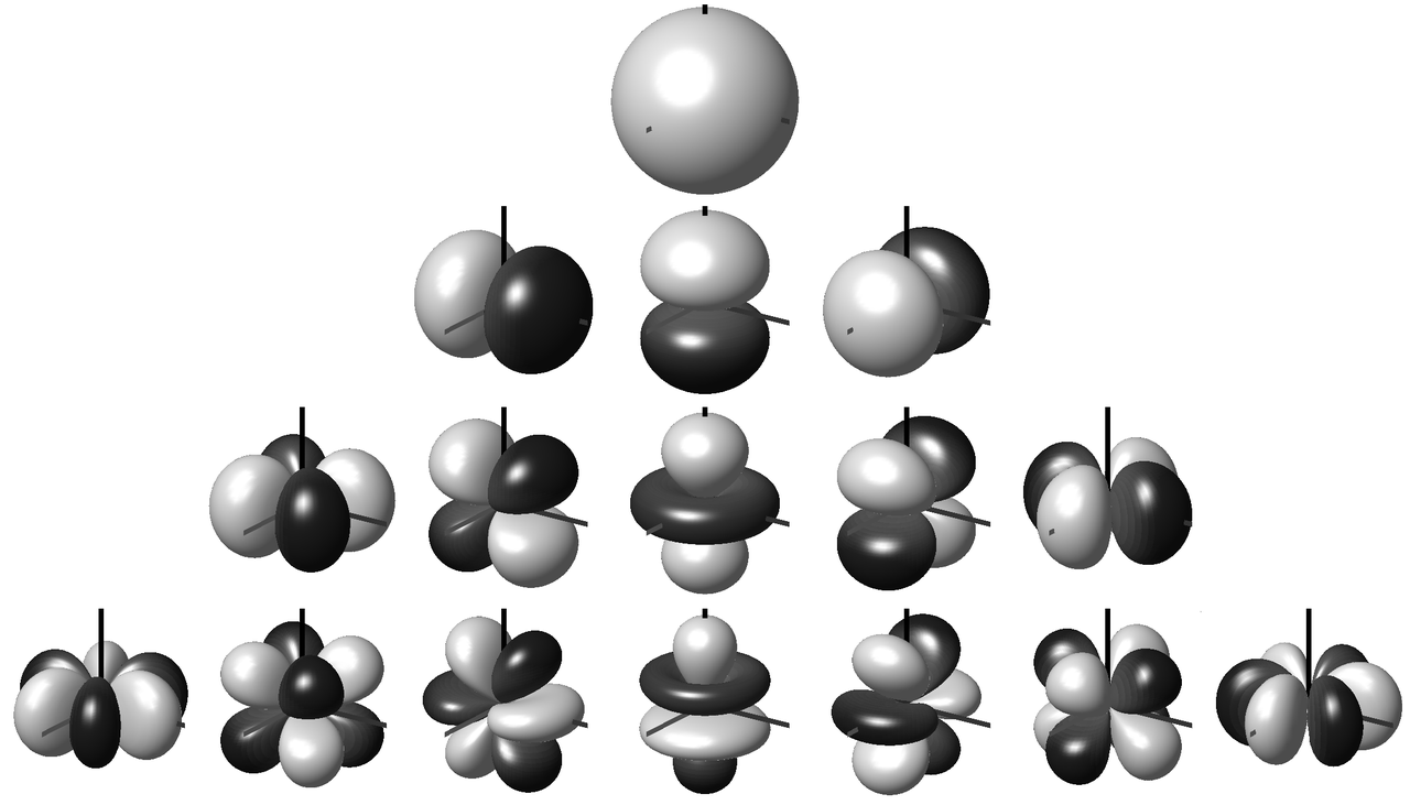
Fig. 1: Spherical harmonics up to order 3 [1].
Ambisonic Formats
An Ambisonics B Format file or signal carries all $N$ spherical harmonics. Figure 2 shows a first order B Format signal.
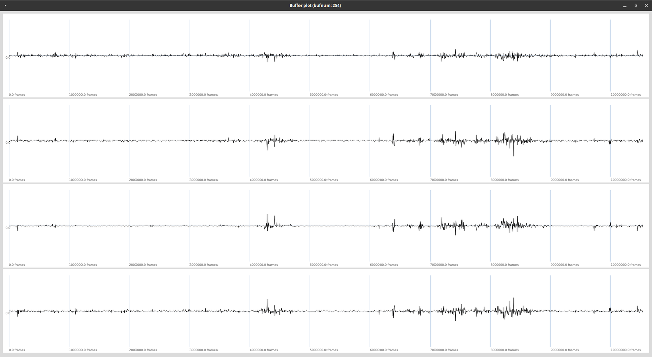
Fig. 2: Four channels of a first order Ambisonics signal.
There are different conventions for the sequence of the individual signals, as well as for the normalization.
FOA / HOA Encoding from Angular Direction
Conventions
Coordinates: \(x=\text{front}\), \(y=\text{left}\), \(z=\text{up}\).
Angles: azimuth \(\varphi \in (-\pi, \pi]\) (CCW from +x toward +y), elevation \(\theta \in [-\pi/2, \pi/2]\) (up from horizontal plane).
Normalisation/order: AmbiX (ACN channel order, SN3D normalisation), unless noted. ACN index \(n=\ell(\ell+1)+m\). For FOA (order \(\ell=1\)), the mapping is \([n]=[0,1,2,3] \leftrightarrow [W,Y,Z,X]\).
First-Order Ambisonics (FOA, B-format) — Single Point Source
A monophonic source \(s(t)\) at direction \((\varphi,\theta)\) encodes to the FOA vector \(\mathbf a(t)=\begin{bmatrix}W&Y&Z&X\end{bmatrix}^{\mathsf T}\) (AmbiX ordering) as:
with the real SN3D first-order spherical harmonics:
Thus, explicitly:
FuMa (legacy) mapping (if required):
FOA — Multiple Point Sources (Object-Based)
For \(N\) sources \(s_i(t)\) at \((\varphi_i,\theta_i)\), FOA channels are a linear sum:
Higher-Order Ambisonics (General Order \(L\))
Let \(Y_{\ell}^{m}(\theta,\varphi)\) be the real SN3D spherical harmonics with \(\ell=0..L\) and \(m=-\ell..\ell\). For a single source:
For \(N\) sources:
Real SN3D Spherical Harmonics (Definition)
With associated Legendre functions \(P_\ell^m(\cdot)\) and SN3D factor \(N_{\ell m}=\sqrt{\dfrac{(2-\delta_{m0})(\ell-m)!}{(\ell+m)!}}\):
Notes
Plane-wave (far-field) model assumed; for finite distance, multiply by a radial factor \(R_\ell(kr)\) (e.g., NFC-HOA).
For head-tracked playback, rotate the Ambisonic channel vector per order using the spherical-harmonic rotation matrices \(\mathbf D_\ell(\cdot)\) before rendering.
References
2015
- Matthias Frank, Franz Zotter, and Alois Sontacchi.
Producing 3d audio in ambisonics.
In Audio Engineering Society Conference: 57th International Conference: The Future of Audio Entertainment Technology–Cinema, Television and the Internet. Audio Engineering Society, 2015.
[details] [BibTeX▼]
2009
- Frank Melchior, Andreas Gräfe, and Andreas Partzsch.
Spatial audio authoring for ambisonics reproduction.
In Proc. of the Ambisonics Symposium. 2009.
[details] [BibTeX▼]