
Understanding Ambisonics
Mid–Side Stereo: 1D Ambisonics
Mid–Side (MS) stereo can be understood as a one-dimensional decomposition of a sound field along a single horizontal axis and works with the same principle as Ambisonics. MS represents the sound field using:
M (Mid) — an cardioid (or omnidirectional) component
S (Side) — a bidirectional (figure-of-eight) component along the left–right axis
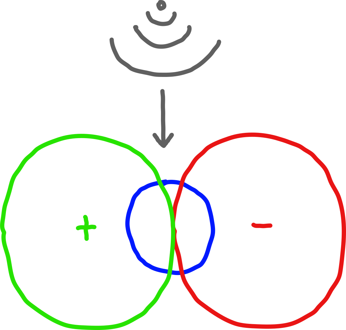
MS configuration with omni (blue) and figure of 8 (greed/red).
This structure already mirrors the first-order Ambisonic idea of decomposing the sound field into orthogonal basis functions.
MS Encoding
Given conventional stereo signals \(L\) and \(R\):
The inverse decoding is:
Interpretation
\(M\) corresponds to an omnidirectional pressure term
\(S\) corresponds to a dipole aligned left–right
The phases of the dipole encode the spatial information.
Mathematically, this is equivalent to a 1D first-order harmonic expansion:
\(M \leftrightarrow Y_0^0\) (monopole)
\(S \leftrightarrow Y_1^{\pm1}\) (horizontal dipole)
In first-order Ambisonics (ACN/SN3D), the related components are:
\(W\) — omnidirectional
\(Y\) — left/right dipole
Matrix Form
MS encoding can also be written as a matrix transform:
and decoding:
A vs B Format
A-format refers to the raw microphone capsule signals (e.g., tetrahedral mic outputs) when capturing 3D sound fields. This format is mic-specific and not interchangeable. To further process it, it usually needs to be converted to B-format. A→B conversion matrices are microphone-model-specific, considering capsule geometry and calibration. Microphone vendors need to supply the decoder.

B-format is made up of the spherical-harmonic components of the sound field. This is the standard Ambisonics format with defined channel order and normalization. B-format is portable and can be reproduced on any rendering system (loudspeaker setups, binaural), following standardized decoding algorithms.
Spherical Harmonics
Basic Ambisonics does not define a sound filed through positions, but through angles of incedence. Ambisonics is based on a decomposition of a sound field into spherical harmonics and dates back to Gerzon's theory of Peryphony (Gerzon, 1973). These spherical harmonics encode a sound field into to different axes, The number of Ambisonics channels $N$ is equal to the number of spherical harmonics. It can be calculated for a given order $M$ with the following formula:
Figure 1 shows the first 16 spherical harmonics. The first row ($N=1$) is the omnidirectional sound pressure for the order $M=0$.
Rows 1-2 together represent the $N=4$ spherical harmonics of the first order Ambisonics signal.
Rows 1-3 correspond to $M=2$, respectively $N=9$.
Rows 1-4 to the third order Ambisonics signal with $N=16$ spherical harmonics.
First order ambisonics is sufficient to encode a threedimensional sound field. The higher the Ambisonics order, the more precise the directional encoding and the better the localization of virtual sound sources.
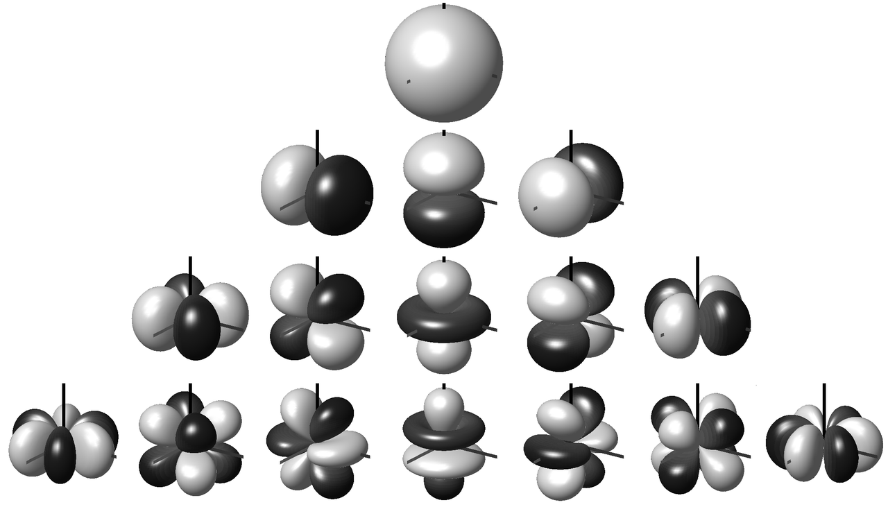
Fig. 1: Spherical harmonics up to order 3 [1].
Common B-format Conventions
B-format conventions define the relation between Ambisonic channel order and spherical harmonics. There are different conventions for the sequence of the individual signals, as well as for the normalization.
| Convention | Type | Channel order (1st order) | Normalization | Notes / Where used |
|---|---|---|---|---|
| FuMa (Furse–Malham) | B-format (FOA) | W, X, Y, Z |
FuMa (“maxN” style; W is scaled by 1/√2) |
Legacy 1st-order B-format used in older DAWs and toolchains; awkward for higher orders (≥2). |
| AmbiX | B-format (FOA/HOA) |
ACN order → [0:W, 1:Y, 2:Z, 3:X]
|
SN3D | De-facto modern production standard (Reaper+AmbiX, many VR/AR SDKs, YouTube VR). Portable and HOA-friendly. |
| ACN/N3D | B-format (FOA/HOA) |
ACN order → [0:W, 1:Y, 2:Z, 3:X]
|
N3D (orthonormal) | Common in research and HOA libraries; convenient for math/analysis and per-order processing. |
Ambisonic Formats
An Ambisonics B Format file or signal carries all $N$ spherical harmonics. Figure 2 shows a first order B Format signal.
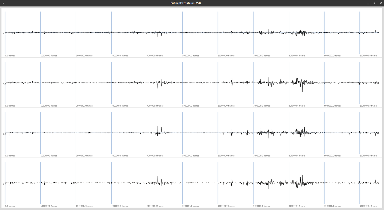
Fig. 2: Four channels of a first order Ambisonics signal.

Fig. 2: Spherical harmonics of a first order Ambisonics signal.
ACN, Normalizations, and 1st-Order Mappings
ACN (Ambisonic Channel Numbering)
The channel index \(n\) is
For 1st order (\(\ell = 0,1\)), the ACN indices map to channels as
Normalizations
SN3D (“semi-normalized”): \(Y_0^0 = 1\). Widely used in production (AmbiX).
-
N3D (fully normalized): spherical harmonics are orthonormal over the unit sphere, i.e.,
\begin{equation*} \int_{S^2} Y_n^m(\Omega)\, Y_{n'}^{m'}(\Omega)\, d\Omega = \delta_{nn'}\,\delta_{mm'} \end{equation*}This normalization yields consistent energy per order and simplifies theoretical work, analysis, and algorithm design in higher-order Ambisonics; however, the order-dependent scaling can increase peak amplitudes in higher orders, requiring additional headroom or gain compensation to avoid clipping in practical implementations.
FuMa (legacy): distinct scaling; notably \(W_{\text{FuMa}} = \tfrac{1}{\sqrt{2}}\,W_{\text{SN3D}}\).
1st-Order Mappings (FuMa ↔ AmbiX/ACN–SN3D)
Channel order
FuMa order:
[W, X, Y, Z]AmbiX (ACN/SN3D) order:
[W, Y, Z, X](i.e., ACN indices[0,1,2,3] -> [W,Y,Z,X])
References
2019
- Franz Zotter and Matthias Frank.
Ambisonics: A Practical 3D Audio Theory for Recording, Studio Production, Sound Reinforcement, and Virtual Reality.
Springer, 2019.
[details] [BibTeX▼]
2015
- Matthias Frank, Franz Zotter, and Alois Sontacchi.
Producing 3d audio in ambisonics.
In Audio Engineering Society Conference: 57th International Conference: The Future of Audio Entertainment Technology–Cinema, Television and the Internet. Audio Engineering Society, 2015.
[details] [BibTeX▼]
2009
- Frank Melchior, Andreas Gräfe, and Andreas Partzsch.
Spatial audio authoring for ambisonics reproduction.
In Proc. of the Ambisonics Symposium. 2009.
[details] [BibTeX▼]
1973
- Michael A. Gerzon.
Periphony: With-Height Sound Reproduction.
Journal of the Audio Engineering Society, 21(1):2–10, 1973.
[details] [BibTeX▼]