Extensions & Plugins for SuperCollider

sc3-plugins

The sc3-plugins are a collection of unit generators (UGen), developed by the SC community. For using the full potential of SuperCollider, it is recommended to install them alongside every SC install:

https://github.com/supercollider/sc3-plugins

The sc3-plugins also contain the SC-HOA UGens, which are needed for working with binaural and Ambisonics in SC.


Extensions

Extra classes are organized in so called Quarks:

https://github.com/supercollider-quarks/quarks

Some addons for SuperCollider require plugins AND extensions. Quarks can be added via code. This example shows how to install the SC-HOA quarks (https://github.com/florian-grond/SC-HOA):

Quarks.install("SC-HOA")

// SuperCollider will automatically install the Quarks here:
Quarks.folder; // execute to see the directory

Another way is to use the Quarks GUI:

Quarks.gui

After restarting sclang (recompiling the class library), you can check whether a Quark (SC-HOA) has been installed properly by checking for related help files, which will be installed:

HOAmbiPanner.help

Configuring the Server

Many application scenarios require specific server configurations. The default server options can be adjusted accordingly.


Multi IO

The number of audio inputs and outputs can be defined before booting the server. Especially in multichannel applications - like in spatial audio - this is necessary:

s.options.numInputBusChannels  = 16;
s.options.numOutputBusChannels = 48;

// boot with options
s.boot;

// show all IO channels
ServerMeter(s);

Running Scripts from the Command Line

Executing Complete Scripts

All above examples were used in a live-coding scenario. The commands were executed in blocks or single lines, step after step. For running a complete script, routines can help to keep the server synchronized. In addition, the server needs to be booted before any server-side operations take place. This can be done with different methods.


Wait for Boot

Server.waitForBoot boots a server and, when completed, runs the function passed to it as an argument:

s.waitForBoot({

   // a sine oscillator node with one parameter
   var x = {|freq=1000| Out.ar(0, SinOsc.ar(freq))}.play;

});

Do when Booted

Server.doWhenBooted need the server to be started with an extra command:

s.doWhenBooted({

    // a sine oscillator node with one parameter
    var x = {|freq=1000| Out.ar(0, SinOsc.ar(freq))}.play;

});

s.boot;

Calling sclang from the Terminal

Once a script is executable as a whole, it can be started using sclang in the command line. When the above file is stored as sine_example.scd, it can be started without launching the scide or any other environment :

$ sclang sine_example.scd

Bilinear Transform: RC Lowpass

The bilinear transform is a method for designing digital filters from analog models. More precisely, it brings filters from the Laplace domain to the z-domain. The desired outcome is a difference function, which can be used for the actual filtering process in the discrete time domain.

Passive RC Lowpass

A simple example for the bilinear transform is the RC lowpass:

Transfer Function

The resulting filter has a low pass characteristic with the following frequency response:

In the Laplace domain its transfer function is defined as:

$$ H(s) = \frac{\omega_c}{\omega_c + s} = \frac{1}{1 + \frac{s}{\omega_c}} $$

$s$ represents the Laplace operator

$$ s = \sigma + j \omega $$

and the cutoff frequency of the passive filter is:

$$ \omega_c = \frac{1}{RC} $$

Substitution

For a transform to the z-domain, the Laplace operator $s$ is subsstituted by the $z$ operator:

$$ s = \frac{2}{T}\frac{1-z^{-1}}{1+z^{-1}} $$$$ z = e^{sT} $$

The following steps rearrange the resulting transfer function to be comprised of summands with the factor $z^{-n}$:

$$ \begin{align} % % H(z) = & \frac{\omega_c}{\omega_c + \frac{2}{T} \frac{1-z^{-1}}{1+z^{-1}}} \\ % = & \frac{\frac{T}{2} \omega_c}{ \frac{T}{2} \omega_c + \frac{1-z^{-1}}{1+z^{-1}}} \\ % = & \frac{\frac{T}{2} \omega_c (1+ z^{-1})}{ \frac{T}{2} \omega_c (1+ z^{-1}) + 1-z^{-1}} \\ % = & \frac{\frac{T}{2} \omega_c + \frac{T}{2} \omega_c z^{-1}}{ \frac{T}{2} \omega_c (1+ z^{-1}) + 1-z^{-1}} \\ % = & \frac{\frac{T}{2} \omega_c + \frac{T}{2} \omega_c z^{-1}}{ \frac{T}{2} \omega_c + \frac{T}{2} \omega_c z^{-1} + 1-z^{-1}} \\ % = & \frac{\frac{T}{2} \omega_c + \frac{T}{2} \omega_c z^{-1}}{1 + \frac{T}{2} \omega_c + (\frac{T}{2} \omega_c -1 )z^{-1}} \\ % \end{align} $$

For getting the coefficients of our digital filter, the transfer function needs to meet the following strucutre where $a_0=1$:

$$ H(z) = \frac{b_0 + b_1 z^{-1}}{1+ a_1 z^{-1}} $$

This is achieved by expanding and simplifying:

$$ \begin{align} % % H(z) = & \frac{\frac{T}{2} \omega_c + \frac{T}{2} \omega_c z^{-1}}{ \underbrace{ \mathbf{\color{gray} 1 + \frac{T}{2} \omega_c }}_{\text{must be 1}} + \left(\frac{T}{2} \omega_c -1 \right)z^{-1}} \\ % = & \frac{\frac{\frac{T}{2} \omega_c}{ 1 + \frac{T}{2} \omega_c} + \frac{ \frac{T}{2} \omega_c}{ 1 + \frac{T}{2} \omega_c} z^{-1}}{1+ \left(\frac{\frac{T}{2} \omega_c}{1 + \frac{T}{2} \omega_c} - \frac{1}{1 + \frac{T}{2} \omega_c} \right)z^{-1}} \\ % = & \frac{\frac{\frac{T}{2} \omega_c}{ 1 + \frac{T}{2} \omega_c} + \frac{ \frac{T}{2} \omega_c}{ 1 + \frac{T}{2} \omega_c} z^{-1}}{1+ \left(\frac{\frac{T}{2} \omega_c -1}{ \frac{T}{2} \omega_c + 1} \right)z^{-1}} \\ \end{align} $$

Coefficients

Following the above rearrangements, the coefficients can be directly extracted from the transfer funcion:

$$ H(z) = \frac{\frac{\frac{T}{2} \omega_c}{ 1 + \frac{T}{2} \omega_c} + \frac{ \frac{T}{2} \omega_c}{ 1 + \frac{T}{2} \omega_c} z^{-1}}{1+ \left(\frac{\frac{T}{2} \omega_c -1}{ \frac{T}{2} \omega_c + 1} \right)z^{-1}} = \frac{b_0 + b_1 z^{-1}}{1+ a_1 z^{-1}} $$$$ \begin{align} \mathbf b_0 = & \frac{\frac{T}{2} \omega_c}{ 1 + \frac{T}{2} \omega_c} \\ \mathbf b_1 = & \frac{\frac{T}{2} \omega_c}{ 1 + \frac{T}{2} \omega_c} \\ \mathbf a_1 = & \frac{\frac{T}{2} \omega_c -1}{ \frac{T}{2} \omega_c + 1} \\ \end{align} $$

Filter Topology

The original dependence of the electrical components R and C is not important at this point. However, with $\omega_c$ = $2 \pi f_0$ we can get the exact coefficients for any cutoff frequency which can be used for the difference equation or applied in the following topology:

Plot Poles and Zeros in Z-Plane

SuperCollider: Synchronous vs Asynchronous

The Problem

Most examples in this class can not be run as a complete script. They need to be evaluated line by line or block wise. One reason for this is the difference between synchronous and asynchronous execution. This problem is in detail explained in the SC guides: https://doc.sccode.org/Guides/Sync-Async.html This site just gives a shorter answer.

Issues usually arise, when a command has been sent to the server and following command depends on the completion of that action. Examples can be the creation of nodes or the loading and filling of buffers. Running this simple block at once will result in an error. It creates a node and does not wait for completion before it uses the .set() method. The result is a FAILURE IN SERVER /n_set Node 1000 not found:

(

// create white noise node with gain control
~test = {arg gain=1; WhiteNoise.ar(gain)}.play;

// try to set the gain
~test.set(\gain, 0.1);

)

A Solution

There are several ways of dealing with the above introduced problem. One solution is to wrap the code block in a Routine, which allows to control the order of execution. In the case of asynchronous tasks, the command s.sync can be used inside a routine. It waits for the sever to finish all asynchronous tasks and the below example works without errors:

(
Routine({

    // create white noise node with gain control
    ~test = {arg gain=1; WhiteNoise.ar(gain)}.play;

    // wait for the server to finish all asynchronous tasks
    s.sync;

    // try to set the gain
    ~test.set(\gain, 0.1);

}).play
)

IIR Filters

Infinite Impulse Response (IIR) filters are such filters which include recursion, respectively feedback, in their implementation. Their impulse response does thus not drop to zero after a given time. They can become instable due to the feedback. However, IIR filters require less coefficients and thus less operations to get a filter with the desired effect than FIR filters. As FIR filters, IIR filters create an output sequence $y[n]$ from an input sequence $x[n]$:

The Difference Equation

For the difference equation the recursion is included with additional coefficients $a_n$, feeding back the output signal $y[n]$ with different delays. The following difference function represents a second order IIR filter. Also referred to as biquad filter, this is a basic component for many digital filter implementations:

$$ y[n] = b_0 x[n] + b_1 x[n-1]+ b_2 x[n-2] - a_1 y[n-1] - a_2 y[n-2] $$

Or short:

$$ y[n] = \sum\limits_{i=0}^{i=N} b_i x[n-i] - \sum\limits_{i=1}^{i=N} a_i y[n-i] $$

Implementation Structure

The above difference equation can be transferred into different implementation structures. These structures can be directly implemented in actual code. The following one is the direct form 1:

Polynominals

A filter of the order $N$ can be expressed as a polynominal, using the Z-operator $z = e^{sT}$:

$$ h[n] = \frac{\sum\limits_{n=0}^{n=N} b_n z^{-n}}{\sum\limits_{n=1}^{n=N} a_n z^{-n}} $$

Pole-Zero Plot

IIR filters have roots in the demoninator, called zeros and in the nominator, called poles:

SuperCollider: Buffers & Samples

Buffers are a tool to hold data arrays on the server and can be used for recording, loading and playing audio files (SC Documentation on Buffers).

SuperCollider comes with a couple of builtin audio samples, which are used in most of the SC helpfiles and examples. The following snippets work with extra audio samples that can be downloaded here: http://ringbuffer.org/download/audio/MFB-522/ They need to be located in the current SC working directory.


Reading Mono Files

The following code creates a client-side object b, that points to a buffer on the default server s - and loads the wav-file kick_1.wav into the buffer:

b = Buffer.read(s, 'kick_1.wav');

When the wav-file has been read, we can get information on the buffer and the sample inside. Like nodes and buses, buffers are known to the server only by their index - the buffer number. We can query this buffer's number:

b.bufnum

There is more information we can get about the sample once it is loaded on the server:

b.numChannels;
b.sampleRate;
b.numFrames;
b.path;

Single Shot Sampler

The sampled audio file in a buffer can be played with the PlayBuf UGen. Since the wav's sample rate and the sample rate of the SC server are not necessarily the same, we need to take care that the playback-rate is adjusted accordingly. The buffer-to-server ration can be calculated in the language (b.sampleRate/s.sampleRate) or using a dedicated UGen:

// PlayBuf args: numChannels, buffer (buffer number), rate
x = {Out.ar(0, PlayBuf.ar(1, b, BufRateScale.kr(b))) }.play;

Note that the node remains on the server and needs to be freed with x.free.


Simple GUI

SuperCollider comes with a simple Qt GUI framework to create functional user interfaces with little effort. The comprehensive SuperCollider GUI Introduction includes many details on the use and customization of GUI elements.

This example usees a slider to control a parameter of a sine oscillator and a button to trigger a noise burst:

(
// a sine oscillator node with one parameter
var x = {|freq=100| Out.ar(0, SinOsc.ar(freq))}.play;

// create a window with width and position
var w = Window("Slider", Rect(128, 64, 800, 480));

// add a slider
var button = Button(w, Rect(400,50,200,200));

// add a slider
var slider = Slider(w, Rect(10,300,1000,100));

// the callback function on slider move
slider.action_({x.set(\freq, pow(slider.value,4) * 10000)});

button.mouseDownAction = {{Out.ar(0, EnvGen.ar(Env([1,0],[1],'lin'),doneAction:Done.freeSelf) * WhiteNoise.ar())}.play};
// same as button.mouseDownAction_(...)

w.fullScreen;
// "same effect as setting -visible to true"
w.front;

)

Exercises

Max: Controlling a Servo

Based on the Arduino-Servo-Example, Max can be used to send control data via USB.


Breadboard Wiring

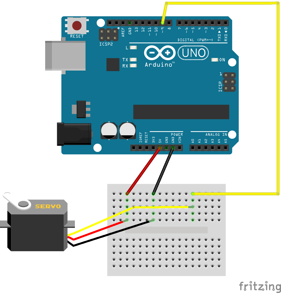
Connecting the servo motor to the Arduino requires no additional parts, except for jumper cables. It is directly powered from the Arduino's 5V pin (larger servos may require an additional power source) and receives data from the Pulse-With-Modulation pin ~9:

Arduino breadboard wiring for servo motor.

Arduino breadboard wiring for servo motor.


Max Patch

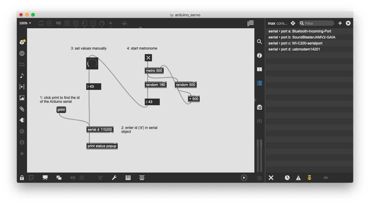
First, find the Arduino's serial port ID by clicking print and enter the result into the serial object (in this case 'd' for 'usbmodem'). The rotary knob can be used to manually set the angle - it needs to be scaled from 0 to 180 before. Finally, the metro can be started with the toggle. It sets random values at randomized time intervals.

Max patch for controlling the servo motor.

Max patch for controlling the servo motor.


Exercise