In the following example, a sine wave's frequency can be changed with an upper limit of $10\ \mathrm{kHz}$.
Depending on the sample frequency of the system running the browser, this will lead to aliasing, once the
frequency passes the Nyquist frequency:
In digital signal processing, sampling refers to the process of converting an analog signal into the digital domain.
A sampled signal will be time-discrete and quantized.
Mathematically, a continuous signal $x(t)$ is sampled by a multiplication with an
impulse train $\delta_T(t)$ (also referred to as Dirac comb) of infitite length:
Since the spectrum of a sampled signal is periodic,
it must be band-limited, in order to avoid misinterpretations,
known as aliasing. Since the spectrum is periodic with $\omega_s$,
the maximum frequency which can be represented - the Nyquist frequency -
is:
$f_N = \frac{f_s}{2}$
As soon as components of a digitally sampled signal exceed this boundary,
aliases occur.
The following example can be used to set the frequency of a sine wave beyond the Nyquist frequency, resulting in aliasing and ambiguity, visualized in the time domain.
The static version of the following example shows the time-domain signal
of a $900 \ \mathrm{Hz}$ sinusoid at a sampling rate $f_s = 1000 \ \mathrm{Hz}$:
For pure sinusoids, aliasing results in a sinusoid
at the mirror- or folding frequency $f_m$:
$f_m = \Big| f - f_s \Big\lfloor \frac{f}{f_s} \Big\rfloor \Big|$
With $\lfloor x \rfloor$ as round to next integer.
At a sampling rate $f_s = 1000 \ \mathrm{Hz}$ and a Nyquist frequency
$f_N = 500 \ \mathrm{Hz}$, a sinusoid with $f = 900 \ \mathrm{Hz}$
will be interpreted as one with $f = 100 \ \mathrm{Hz}$:
f_m = 100
The following example can be used interactively as a Jupyter notebook,
by changing the frequency of a sinusoid and listening to the aliased
output. When sweeping the range up to $2500 \ \mathrm{Hz}$, the
resulting output will increase and decrease in frequency.
In the static version, a sinusoid of $f = 900 \ \mathrm{Hz}$
is used, resulting in an audible output at $f_m = 100 \ \mathrm{Hz}$:
For signals with overtones, undersampling leads to inharmonic
alisases and happen before the fundamental itself exceeds
the Nyquist frequency.
For a harmonic signal with a fundamental frequeny $f_0$,
the alias frequencies for all $N$ harmonics can be calculated:
For certain fundamental frequencies, all aliases will be located at actual
multiples of the fundamental, resulting in a correct synthesis despite aliasing.
The following example uses a sampling rate $f_s = 16000 \ \mathrm{Hz}$,
with an adjustable $f_0$ for the use as a Jupyter notebook.
In the static HTML version, a square wave of $f_0 = 277 \ \mathrm{Hz}$
is used and the result with aliasing artefacts can be heard.
The plot shows the additional content caused by the mirror frequencies:
In analog-to-digital conversion, simple anti-aliasing filters can be used
to band-limit the input and discard signal components above the Nyquist frequency.
In case of digital synthesis, however, this principle can not
be applied. When generating a square wave signal with an infinite
number of harmonics, aliasing happens instantaneoulsy and can not be
removed, afterwards.
The following example illustrates this, by using a 5th order Butterworth
filter with a cutoff frequency of $f_c = 0.95 \frac{f_s}{2}$. Although the output
signal is band-limited, the aliasing artifacts are still contained
in the output signal.
  Cell In[10], line 3
    In order to avoid aliasing problems, most environments for audio signal processing and
       ^
SyntaxError: invalid syntax
Python can be used inside virtual environments.
A venv is treated like an isolated Python install.
Virtual environments can be activated and deactivated.
When activated, the interpreter will only work with the modules and packages installed specifically
in this venv.
This makes it easier to work on multiple projects with different required packages.
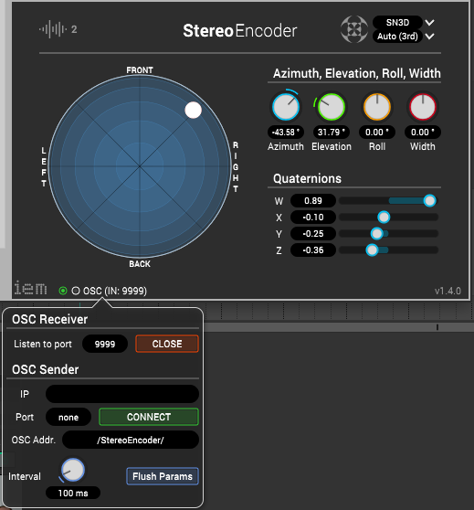
Controlling the IEM plugins with OSC messages, i.e. sent from another software or expressive interfaces, opens more possibilities than using only DAW automations. Each plugin in the suite comes with a OSC receiver, which can be enabled and listens to a defined set of messages.
All information for controlling the IEM plugins, including the defined OSC paths are included in the IEM documentation: https://plugins.iem.at/docs/osc/
The following example shows how to control the position of a virtual sound source, using the StereoEncoder plugin.
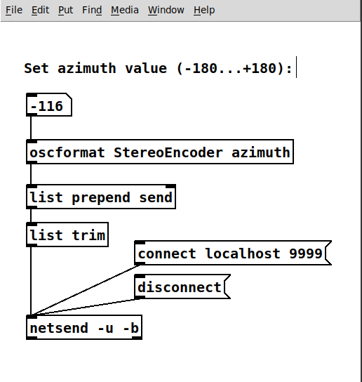
The following PD patch uses no additional libraries and should work as it is. Both the IEM plugins and PD need to me running on the same machine. It snds to a port via netsend (click connect to localhost in the beginning) - it needs to be the same one opened by the plugin.
The OSC path is defined in the oscformat object. It can be changed, if other paramters should be controlled.
NOTE:
Since a single encoder plugin opens an individual OSC port, each instance of the encoder plugin needs to open an individual port. The MultiEncoder allows the control of more sources (but in one channel). with a single port.
Max's Live Object Model makes it possible to exchange data between
Max for Live and any parameter of a Live session.
The model is best described in the
Max Online Documentation.
and the
Live API Overview
In the following examples, different Live parameters are controlled via
LFOs or direct input to demonstrate the capabilities.
The Live Object Model
Working with the Live Object Model involves four objects:
The live.path object is used to select objects in the Live object hierarchy. It receives a message, pointing to the object which is to be accessed.
live.object is used to get and set properties and children of objects and to call their functions.
The live.observer object can subscribe to properties of objects and their children and gets regular updates on changes.
With the live.parameter~ object it is possible to control Live device parameters in real time.
Controlling the Live Set
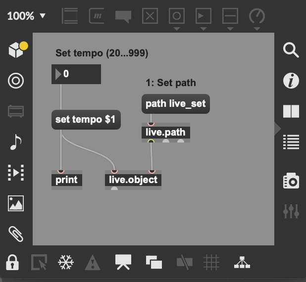
This first example allows to change the playback speed of the Live session in BPM.
The live object only needs the path to the Live set (live_set) and
can then process the set tempo $1 message.
Setting the session tempo from Max for Live.
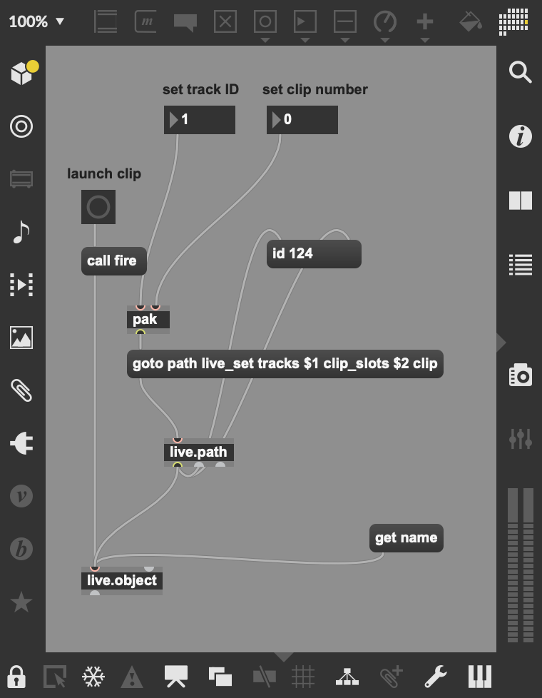
Triggering Clips
Each clip in Live's session view can be accessed with an individual path.
Once set with the goto ... message, the call fire message can trigger the sample.
Launching the first clip of the second channel from Max for Live.
This tutorial gives more insight on controlling all clip properties offered by Live: Hack Live 11 Clip Launching
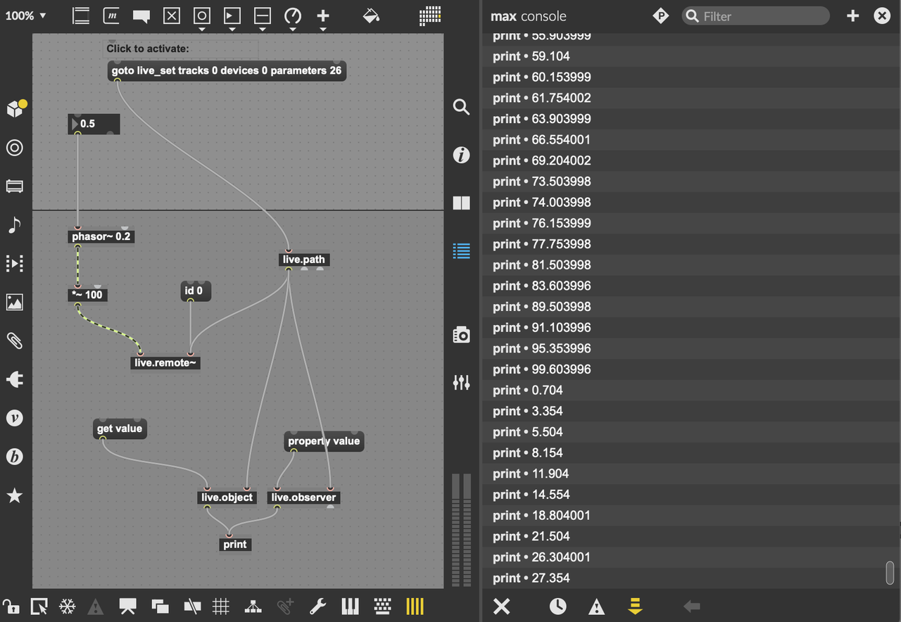
Controlling Device Parameters
By controlling device parameters, any synth or effect inside a Live
project can be automated from Max For Live patches.
Although this is a very powerful feature, paths to the objects need to be tracked
down by the indices of the channel, the plugin and the parameter.
Instrument Channels
In this example, the Granulator II is used. It can be installed via
the Ableton Website.
The first thing to do is find the right path for the device and parameter.
oköas .
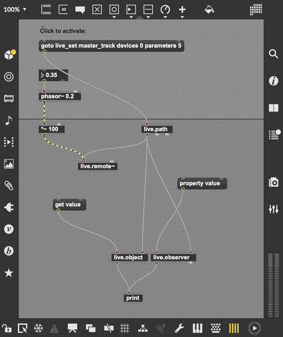
Main Channel
Main channel effects and plugins can be controlled in the same way as those in instrument channels,
omitting the channel index.
Patch for controlling the cutoff frequency of a filter in the main channel.
There is a variety of different approaches for receiving (and sending) data via a serial port in PD.
The solution in this example relies OSC via serial and needs additional libraries for both the Arduino sender
and the PD receiver.
In return it offers a flexible approach for handling multiple sensors.
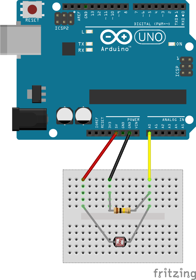
Breadboard Circuit
The breadboard circuit is the same as in the first Arduino sensor example:
Arduino Code
For the following Arduino program, the additional OSC Library by Adrian Freed
needs to be installed. It can be cloned from the repository or simply installed with
the builtin package manager in the Arduino IDE (Tools->Manage Libraries).
OSCMessage.h is included in the code.
In addition, the type of serial connection is retrieved.
The OSCMessage class is used in the main loop to pack the data and send it.
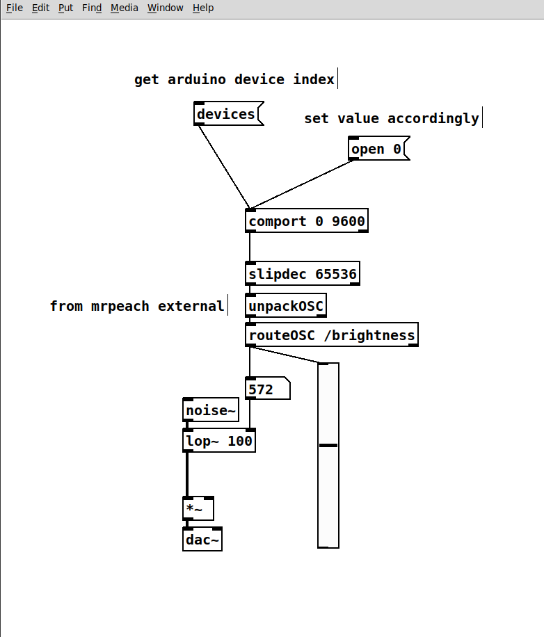
The Pure Data receiver patch relies on the mrpeach externals: mrpeach GitHub Repository
Like many externals, they can be installed by cloning the repository to one of PD'2 search paths - or by using Deken. The external is named mrpeach: Instructions for using Deken
Serial data is received with the comport object. All available devices can be printed
to PD's console. The proper interface can be opened with an extra message or as
first argument of the object. On Linux systems, this is usually /dev/ttyACM0.
The slipdec object decodes the SLIP-encoded OSC message, which is then
unpacked and routed.
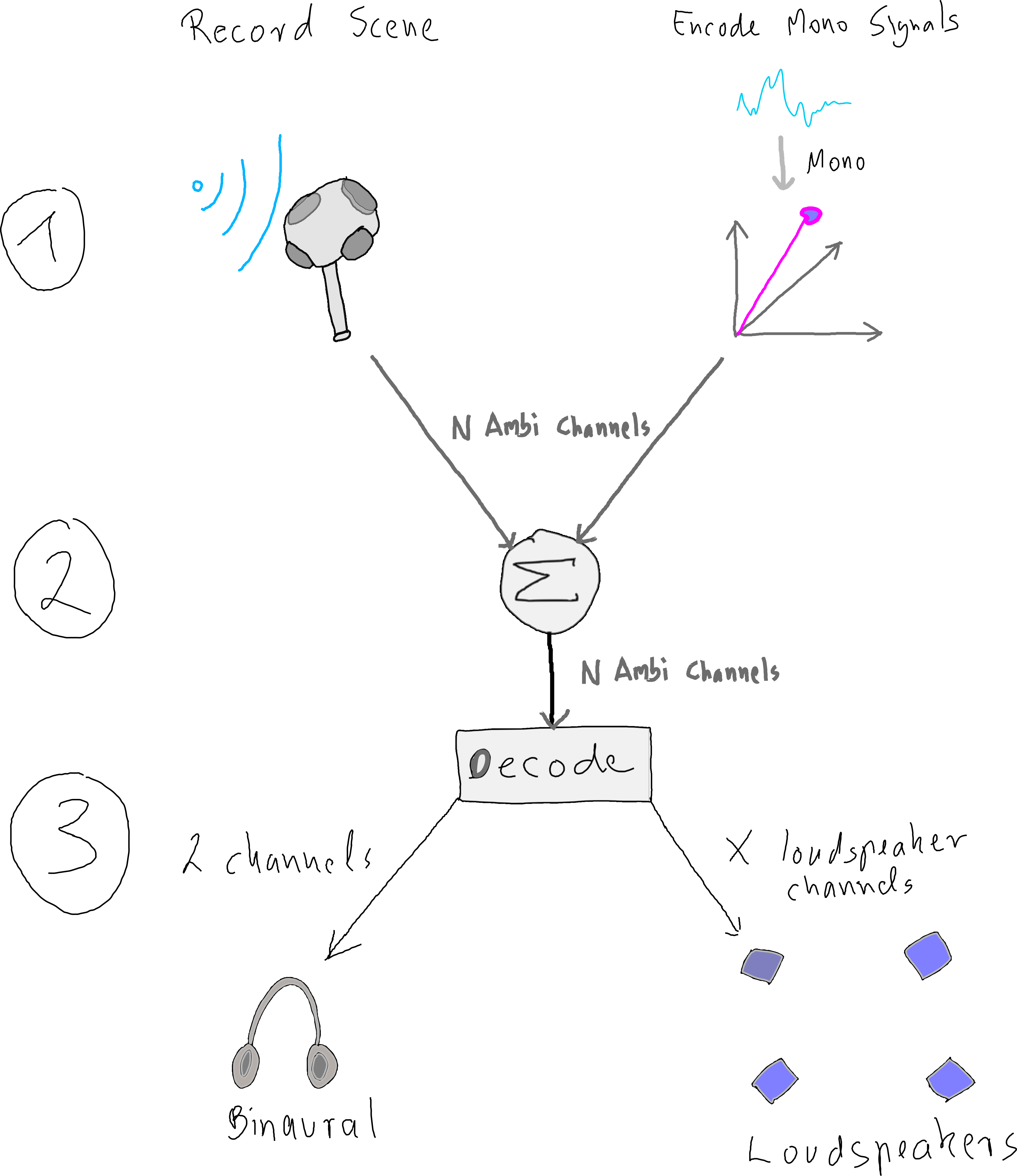
A basic Ambisonics production workflow can be split into three stages, as shown in Figure 1.
The advantage of this procedure ist that the production is independent of the output format,
since the intermediate format is in the Ambisonics domain.
A sound field produced in this way can subsequently be rendered or decoded to any desired
loudspeaker setup or headphones.
Figure 1: Basic Ambisonics production workflow.
Stages
1: Encoding Stage
In the encoding stage, Ambisonics signals are generated. This can happen via recording with an
Ambisonics microphone or through encoding of mono sources with individual angles (azimuth, elevation).
A plain Ambisonics encoding does not include distance information - altough it can be added through attenuation.
All encoded signals have the same amount of $N$ ambisonics channels.
2: Summation Stage
All individual Ambisonics signals can be summed up to create one scene,
respectively one sound field.
3: Decoding Stage
In the decoding stage, individual output signals can be calculated. This requires either
head-related transfer functions or loudspeaker coordinates.
More advanced workflows may feaure additional stages for manipulating encoded Ambisonics signals,
inlcuding directional filtering or rotation of the audio scene.
References
2015
Matthias Frank, Franz Zotter, and Alois Sontacchi.
Producing 3d audio in ambisonics.
In Audio Engineering Society Conference: 57th International Conference: The Future of Audio Entertainment Technology–Cinema, Television and the Internet. Audio Engineering Society, 2015. [details]
[BibTeX▼]
@inproceedings{frank2015producing,
    author = "Frank, Matthias and Zotter, Franz and Sontacchi, Alois",
    title = "Producing 3D audio in ambisonics",
    booktitle = "Audio Engineering Society Conference: 57th International Conference: The Future of Audio Entertainment Technology--Cinema, Television and the Internet",
    year = "2015",
    organization = "Audio Engineering Society"
}
@inproceedings{melchior2009spatial,
    author = {Melchior, Frank and Gr{\"a}fe, Andreas and Partzsch, Andreas},
    title = "Spatial audio authoring for Ambisonics reproduction",
    booktitle = "Proc. of the Ambisonics Symposium",
    year = "2009"
}
Additive Synthesis and Spectral Modeling are in detail introduced in the
corresponding sections of the
Sound Synthesis Introduction.
Since sounds are created by combining large numbers of spectral components, such as harmonics
or noise bands, spatialization at synthesis stage is an obvious method.
Listeners can thereby be spatially enveloped by a single sound,
with spectral components being perceived from all angles.
The continuous character, however, blurs the localization.
SOS
Spatio-operational spectral (SOS) synthesis (Topper, 2002) is an attempt towards a
dynamic spatial additive synthesis, implemented in MAX/MSP and RTcmix.
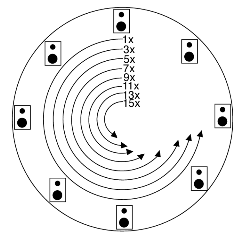
Partials are rotated independently within a 2D 8 channel speaker setup.
A first experiment used a varying rate circular spatial path of
the first eight partials of a square wave, as shown in Figure 1.
Figure 1: First SOS experiment (Topper, 2002).
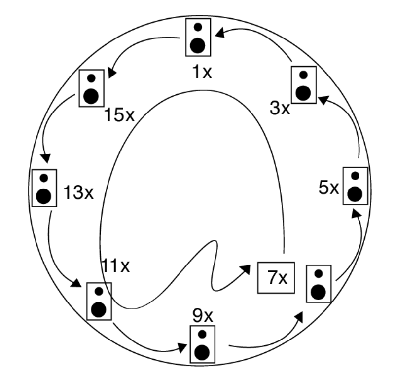
Figure 2 shows the second experiment with one partial moving against the
others.
Figure 2: Second SOS experiment (Topper, 2002).
GLOOO
GLOOO is a system for real-time expressive spatial synthesis with spectral
models.
A haptic interface allows the dynamic distribution of 100 spectral components,
allowing a control over the spread and position of the resulting violin sound.
The project is best documented on the corresponding websites:
@inproceedings{grimaldi2017parametric,
    author = {{Grimaldi, Vincent and B{\"o}hm, Christoph and Weinzierl, Stefan and von Coler, Henrik}},
    booktitle = "{Proceedings of the 142nd Audio Engineering Society Convention}",
    location = "Berlin, Germany",
    organization = "Audio Engineering Society",
    title = "{Parametric Synthesis of Crowd Noises in Virtual Acoustic Environments}",
    year = "2017"
}
@inproceedings{james2015spectromorphology,
    author = "James, Stuart",
    booktitle = "{Proceedings of the International Computer Music Conference (ICMC)}",
    location = "Denton, Texas, United States",
    title = "Spectromorphology and Spatiomorphology of Sound Shapes: audio-rate {AEP} and {DBAP} panning of spectra",
    year = "2015"
}
@inproceedings{mcgee2015spatial,
    author = "McGee, Ryan",
    booktitle = "{Proceedings of the International Computer Music Conference (ICMC)}",
    location = "Denton, USA",
    title = "Spatial Modulation Synthesis",
    year = "2015"
}
@inproceedings{muller2009physical,
    author = {M{\"u}ller, Alexander and Rabenstein, Rudolf},
    booktitle = "{Proceedings of the International Conference of Digital Audio Effects (DAFx)}",
    location = "Como, Italy",
    title = "Physical Modeling for Spatial Sound Synthesis",
    year = "2009"
}
@inproceedings{wilson2008spatial,
    author = "Wilson, Scott",
    booktitle = "{Proceedings of the International Computer Music Conference (ICMC)}",
    location = "Belfast, Ireland",
    title = "Spatial Swarm Granulation",
    year = "2008"
}
@inproceedings{kim2008spectral,
    author = "Kim-Boyle, David",
    address = "Belfast, UK",
    booktitle = "{Proceedings of the International Computer Music Conference (ICMC)}",
    title = "Spectral Spatialization - an Overview",
    year = "2008"
}
2004
Curtis Roads.
Microsound.
The MIT Press, 2004.
ISBN 0262681544. [details]
[BibTeX▼]
@book{roads2004microsound,
    author = "Roads, Curtis",
    isbn = "0262681544",
    publisher = "The MIT Press",
    title = "{Microsound}",
    year = "2004"
}
@inproceedings{topper2003spatio,
    author = "Topper, David and Burtner, Matthew and Serafin, Stefania",
    address = "Singapore",
    booktitle = "{Proceedings of the International Conference of Digital Audio Effects (DAFx)}",
    location = "Hamburg, Germany",
    title = "Spatio-Operational Spectral ({SOS}) Synthesis",
    year = "2002"
}
The Klangmühle was an early electronic device for spatialization, allowing the
panning between different channels by moving a crank, which was then mapped to multiple variable resistors.
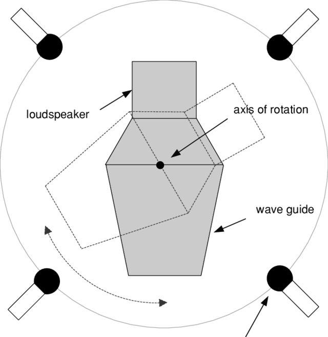
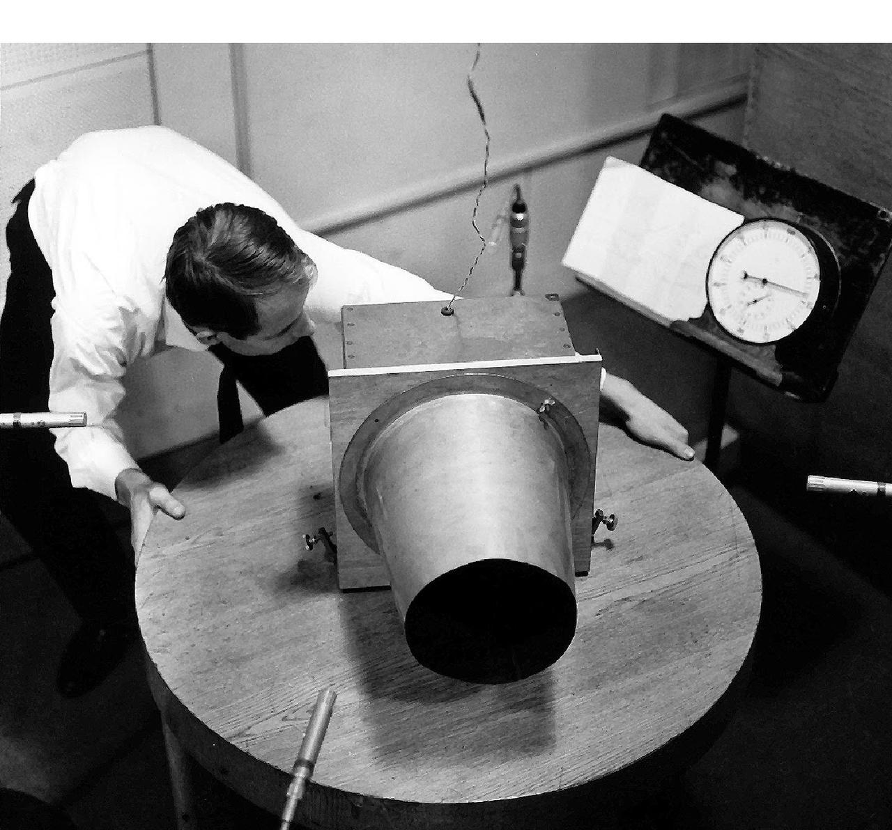
Rotationstisch
The Rotationstisch was used by Karlheinz Stockhausen for his work Kontakte (1958-60) (von Blumroeder, 2018).
In the studio, the device was used for producing spatial sound movements on a quadraphonic loudspeaker setup.
This was realized with four microphones in a quadratic setup, each pointing towards a loudspeaker in the center:
Functional sketch of the Rotationstisch (Braasch, 2008).
The predominant effect of the Rotationstisch is amplitude panning, using the directivity of the loudspeaker and wave guide. In addition,
the spatialization includes a Doppler shift when rotating the loudspeaker. The rotation device can be moved manually, thus allowing to perform
the spatial movements and record them on quadraphonic tape:
Rotationstisch , operated by Karlheinz Stockhausen (Stockhausen-Stiftung für Musik, Kürten).
Kontakte
Stockhausen's 1958-60 composition Kontakte can be considered a milestone of multichannel music.
It exists as a tape-only version, as well as a version for tape and live piano and percussion.
For the tape part, the Rotationstisch was used to create the spatial movements - not
fully captured in this stereo version (electronics only).
Listen to 17'00'' for the most prominent rotation movement in four channels:
Composing within the electronic medium, i. e. modifying sound with the help of electroacoustic apparatuses, has been an essential determinating factor in the musical work of Karlheinz Stockhausen, as a spectrum of electronic pieces from Studie I (1953) to Kontakte (1958-60), Mixtur (1964), Hymnen (1966-67), Oktophonie (1990/91), and Cosmic Pulses (2007) documents. The article considers this seemingly well-known fact from a revised musicological perspective. Considerations from a broader compositional-creative context that include both instrumental and vocal components lead to insights into the origins and history of some of Stockhausen's electronic projects that have found less attention until now.
@article{vonblumroeder2018zurbedeutung,
    author = "Blumröder, Christoph von",
    journal = "Archiv für Musikwissenschaft",
    number = "3",
    pages = "166–178",
    publisher = "Franz Steiner Verlag",
    title = "Zur Bedeutung der Elektronik in Karlheinz Stockhausens Œuvre / The Significance of Electronics in Karlheinz Stockhausen's Work",
    volume = "75",
    year = "2018"
}
@incollection{vonColer2015aspects,
    author = "Brech, Martha and von Coler, Henrik",
    editor = "Brech, Martha and Paland, Ralph",
    booktitle = "Compositions for Audible Space",
    pages = "193--204",
    publisher = "transctript",
    series = "{Music and Sound Culture}",
    title = "Aspects of Space in {Luigi Nono's Prometeo} and the use of the {Halaphon}",
    year = "2015"
}
@inproceedings{chowning2011turenas,
    author = "Chowning, John",
    booktitle = "{Proceedings of the 17th Journ{\'e}es d{\rq}Informatique Musicale}",
    location = "Saint-Etienne, France",
    title = "Turenas: The Realization of a Dream",
    year = "2011"
}
@article{moormann2010raum,
    author = "Moormann, Peter",
    doi = "doi:10.1524/para.2010.0023",
    url = "https://doi.org/10.1524/para.2010.0023",
    title = "Raum-Musik als Kontaktzone. Stockhausens Hymnen bei der Weltausstellung in Osaka 1970",
    journal = "Paragrana",
    number = "2",
    volume = "19",
    year = "2010",
    pages = "33--43"
}
@article{braasch2008aloudspeaker,
    author = "Braasch, Jonas and Peters, Nils and Valente, Daniel",
    year = "2008",
    month = "09",
    pages = "55-71",
    title = "A Loudspeaker-Based Projection Technique for Spatial Music Applications Using Virtual Microphone Control",
    volume = "32",
    journal = "Computer Music Journal"
}