Wavefolding

Wavefolding

Wavefolding is a special case of waveshaping, working with periodic transfer functions. Depending on the pre-gain, the source signal gets folded back, once a maximum of the transfer function is reached. Compared to the previously introduced soft clipping or other methods of waveshaping, this adds many strong harmonics.

Periodic Shaping Function

A simple basic transfer function is a sine with the appropriate scaling factor. The pre-gain $g$ is the parameter for controling the intensity of the folding effect:

$$ y[n] = sin( g \frac{\pi}{2} x[n]) $$

For an input signal $x$, limited to values between $-1$ and $1$, respectively for gains $g\leq1$, this results in a sinusoidal waveshaping function with saturation:

Text(0,0.5,'y')

When the input signal exceeds the boundaries $-1$ and $1$, the signal does not clip but is folded back. This can be achieved by amplifying the input with an additional gain:

For a gain of $g=3$, the time-domain output signal looks as follows:

Spectrum for a Sinusoidal Input

The spectrum of wavefolding can be calculated by expressing the folding term as a Fourier series: The Jacobi–Anger expansion can be used for this purpose, with the pre-gain $g$:

$$ \sin(g \sin(x)) = 2 \sum\limits_{m=1}^{\infty} J_{2m-1}(g) \sin((2m-1)x) $$

At this point it is already apparent that the resulting signal contains harmonics at odd integer multiples of the fundamental frequency $f_m = 100 \mathrm{Hz}\ (2 m -1)$. Their gain is determined by first kind Bessel functions $J_{2m-1}(g)$:

For the DFT this leads to:

$$ \begin{eqnarray} X[k] &=& 2 \sum\limits_{m=1}^{\infty} J_{2m-1}(g) \sin((2m-1)x) \sum\limits_{n=0}^{N-1} e^{-j 2 \pi k \frac{n}{N}} \\ % % % X[k] &=& 2 \sum\limits_{n=0}^{N-1} \sum\limits_{m=1}^{\infty} J_{2m-1}(g) \sin((2m-1)x)\ e^{-j 2 \pi k \frac{n}{N}} \\ % % % X[k] &=& 2 \sum\limits_{n=0}^{N-1} \sum\limits_{m=1}^{\infty} J_{2m-1}(g) \frac{1}{2} \left( e^{j (2m-1)x} - e^{-j(2m-1)x} \right) % \sin((2n-1)x)\ e^{-j 2 \pi k \frac{n}{N}} \\ % % % X[k] &=& \sum\limits_{n=0}^{N-1} \sum\limits_{m=1}^{\infty} J_{2m-1}(g) \left( e^{-j 2 \pi k \frac{n}{N} + j (2m-1)x } - e^{-j 2 \pi k \frac{n}{N} -j(2m-1)x} \right) % \sin((2n-1)x)\ \end{eqnarray} $$

With $x = 2 \pi \frac{f_0}{f_s} n$

$$ X[k] = \sum\limits_{n=0}^{N-1} \sum\limits_{m=1}^{\infty} J_{2m-1}(g) \left( e^{-j 2 \pi k \frac{n}{N} + j (2m-1) 2 \pi \frac{f_0}{f_s} } - e^{-j 2 \pi k \frac{n}{N} -j(2m-1) 2 \pi \frac{f_0}{f_s}} \right) % \sin((2n-1)x)\ $$

1 Hints on this by Peyam Tabrizian can be found here: https://youtu.be/C641y-z3aI0
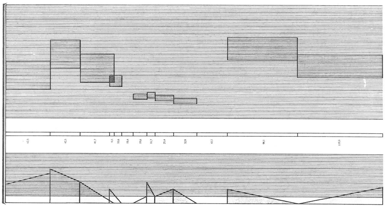
DFT Plots

The below plots show the spectra of the folding operation for a sine input of $100 \mathrm{Hz}$ at different gains. With increasing gain, partials are added at the odd integer multiples of the fundamental frequency $f_m = 100 \mathrm{Hz}\ (2 m -1)$:

[ 100  300  500  700  900 1100 1300 1500 1700 1900] ...

Combining Nodes in SuperCollider

Creating and Connecting Nodes

Audio buses can be used to connect synth nodes. In this example we will create two nodes - one for generating a sound and one for processing it. First thing is an audio bus:

~aBus = Bus.audio(s,1);

The ~osc node generates a sawtooth signal and the output is routed to the audio bus:

~osc = {arg out=1; Out.ar(out,Saw.ar())}.play;

~osc.set(\out,~aBus.index);

The second node is a simple filter. Its input is set to the index of the audio bus:

~lpf = {arg in=0; Out.ar(0, LPF.ar(In.ar(in),100))}.play;

~lpf.set(\in,~aBus.index);

Moving Nodes

/images/basics/sc-order-1.png

Node Tree before moving the processor node.


The moveAfter() function is a quick way for moving a node directly after a node specified as the argument. The target node can be either referred to by its node index or by the related name in sclang:

~lpf.moveAfter(~osc)

/images/basics/sc-order-2.png

Node Tree after moving the processor node.

More APIs

There are many more APIs which can be used for real time or off line sonification. Several projects and meta sites list examples by category:


NASA

NASA offers a great variety of open APIs with data from astronomy: https://api.nasa.gov/


WHO

https://www.who.int/data/gho/info/gho-odata-api


Create an API

https://towardsdatascience.com/a-layman-guide-for-data-scientists-to-create-apis-in-minutes-31e6f451cd2f

Digital Waveguides: Discrete Wave Equation

Wave Equation for Ideal Strings

The ideal string results in an oscillation without losses. The differential wave-equation for this process is defined as follows. The velocity \(c\) determines the propagation speed of the wave and this the frequency of the oscillation.

\begin{equation*} \frac{\partial^2 y}{\partial t^2} = c^2 \frac{\partial^2 y}{\partial x^2} \end{equation*}

A solution for the different equation without losses is given by d'Alembert (1746). The oscillation is composed of two waves - one left-traveling and one right traveling component.

\begin{equation*} y(x,t) = y^+ (x-ct) + y^- (x+ct)$ \end{equation*}
  • \(y^+\) = left traveling wave

  • \(y^-\) = right traveling wave


Tuning the String

The velocity \(c\) depends on tension \(K\) and mass-density \(\epsilon\) of the string:

\begin{equation*} c^2 = \sqrt{\frac{K}{\epsilon}} = \sqrt{\frac{K}{\rho S}} \end{equation*}

With tension \(K\), cross sectional area \(S\) and density \(\rho\) in \({\frac{g}{cm^3}}\).

Frequency \(f\) of the vibrating string depends on the velocity and the string length:

\begin{equation*} f = \frac{c}{2 L} \end{equation*}

Make it Discrete

For an implementation in digital systems, both time and space have to be discretized. This is the discrete version of the above introduced solution:

\begin{equation*} y(m,n) = y^+ (m,n) + y^- (m,n) \end{equation*}

For the time, this discretization is bound to the sampling frequency \(f_s\). Spatial sample distance \(X\) depends on sampling-rate \(f_s = \frac{1}{T}\) and velocity \(c\).

  • \(t = \ nT\)

  • \(x = \ mX\)

  • \(X = cT\)


References

2019

  • Stefan Bilbao, Charlotte Desvages, Michele Ducceschi, Brian Hamilton, Reginald Harrison-Harsley, Alberto Torin, and Craig Webb. Physical modeling, algorithms, and sound synthesis: the ness project. Computer Music Journal, 43(2-3):15–30, 2019.
    [details] [BibTeX▼]

2004

  • Chris Chafe. Case studies of physical models in music composition. In Proceedings of the 18th International Congress on Acoustics. 2004.
    [details] [BibTeX▼]

1995

  • Vesa Välimäki. Discrete-time modeling of acoustic tubes using fractional delay filters. Helsinki University of Technology, 1995.
    [details] [BibTeX▼]
  • Gijs de Bruin and Maarten van Walstijn. Physical models of wind instruments: A generalized excitation coupled with a modular tube simulation platform*. Journal of New Music Research, 24(2):148–163, 1995.
    [details] [BibTeX▼]

1993

  • Matti Karjalainen, Vesa Välimäki, and Zoltán Jánosy. Towards High-Quality Sound Synthesis of the Guitar and String Instruments. In Computer Music Association, 56–63. 1993.
    [details] [BibTeX▼]

1992

  • Julius O Smith. Physical modeling using digital waveguides. Computer music journal, 16(4):74–91, 1992.
    [details] [BibTeX▼]

1971

  • Lejaren Hiller and Pierre Ruiz. Synthesizing musical sounds by solving the wave equation for vibrating objects: part 1. Journal of the Audio Engineering Society, 19(6):462–470, 1971.
    [details] [BibTeX▼]
  • Lejaren Hiller and Pierre Ruiz. Synthesizing musical sounds by solving the wave equation for vibrating objects: part 2. Journal of the Audio Engineering Society, 19(7):542–551, 1971.
    [details] [BibTeX▼]

Faust: MIDI

Using MIDI CC

Using MIDI in Faust requires only minor additions to the code and compiler arguments. For first steps it can be helpful to control single synth parameters with MIDI controllers. This can be configured via the UI elements. The following example uses MIDI controller number 48 to control the frequency of a sine wave by adding [midi:ctrl 48] to the hslider parameters.


// midi-example.dsp
//
// Control a sine wave frequency with a MIDI controller.
//
// Henrik von Coler
// 2020-05-17

import("stdfaust.lib");

freq = hslider("frequency[midi:ctrl 48]",100,20,1000,0.1) : si.smoo;

process = os.osc(freq) <: _,_ ;

CC 48 has been chosen since it is the first slider on the AKAI APC mini. If the controller numbers for other devices are not known, they can be found using the PD patch reverse_midi.pd.


Compiling with MIDI

In order to enable the MIDI functions, the compiler needs to be called with an additional flag -midi:

$ faust2xxxx -midi midi_example.dsp

This flag can also be combined with the -osc flag to make synths listen to both MIDI and OSC.


Note Handling & Polyphony

Typical monophonic and polyphonic synth control can be added to Faust programs by defining and mapping three parameters:

  • freq

  • gain

  • gate

When used like in the following example, they will be linked to the parameters of MIDI note on and note off events with a frequency and a velocity.

// midi_trigger.dsp
//
// Henrik von Coler
// 2020-05-17

import("stdfaust.lib");
freq    = nentry("freq",200,40,2000,0.01) : si.polySmooth(gate,0.999,2);
gain   = nentry("gain",1,0,1,0.01) : si.polySmooth(gate,0.999,2);
gate   = button("gate") : si.smoo;

process = vgroup("synth",os.sawtooth(freq)*gain*gate <: _,_);

Compiling Polyphonic Code

$ faust2xxxx -midi -nvoices 12 midi_trigger.dsp

MIDI on Linux

Faust programs use Jack MIDI, whereas MIDI controllers usually connect via ALSA MIDI. In order to control the synth with an external controller, a bridge is nedded:

$ a2jmidi_bridge

The MIDI controller can now connect to the a2j_bridge input, which is then connected to the synth input.

Faust: Splitting and Merging Signals

Splitting a Signal

To Stereo

The <: operator can be used to split a signal into an arbitrary number of branches. This is frequently used to send a signal to both the left and the right channel of a computer's output device. In the following example, an impulse train with a frequency of $5\ \mathrm{Hz}$ is generated and split into a stereo signal.

text


import("stdfaust.lib");

// a source signal
signal = os.imptrain(5);

// split signal to stereo in process function:
process = signal <: _,_;

To Many

The splitting operator can be used to create more than just two branches. The following example splits the source signal into 8 signals:

text


To achieve this, the splitting directive can be extended by the desired number of outputs:

process = signal <: _,_,_,_,_,_,_,_;

Merging Signals

Merging to Single

The merging operator :> in Faust is the inversion of the splitting operator. It can combine an arbitrary number of signals to a single output. In the following example, four individual sine waves are merged:

text


Input signals are separated by commas and then joined with the merging operator.

import("stdfaust.lib");

// create four sine waves
// with arbitrary frequencies
s1 = 0.2*os.osc(120);
s2 = 0.2*os.osc(340);
s3 = 0.2*os.osc(1560);
s4 = 0.2*os.osc(780);

// merge them to two signals
process = s1,s2,s3,s4 :> _;

Merging to Multiple

Merging can be used to create multiple individual signals from a number of input signals. The following example generates a stereo signal with individual channels from the four sine waves:

text


To achieve this, two output signals need to be assigned after merging:

// merge them to two signals
process = s1,s2,s3,s4 :> _,_;

Exercise

Subtractive Example

The following example uses a continuous square wave generator with different filters for exploring their effect on a harmonic signal.

Controls

Pitch (VCF):

Filter Type:

Lowpass Highpass Bandpass Notch (Band Reject)

Cutoff (VFC):

Q (VCF):

Gain (VCA):

Time Domain Plot

t/s

Frequency Domain Plot

f/Hz

Additive & Spectral: History

Early Mechanical

Early use of the Fourier representation, respectively additive synthesis, for modeling musical sounds has been made by Hermann von Helmholtz. He built mechanical devices, based on tuning forks, resonant tubes and electromagnetic excitation for additive synthesis. Von Helmholtz used these devices for investigating various aspects of harmonic sounds, including spectral distribution and relative phases.

/images/Sound_Synthesis/helmholtz_fork.jpg

Tuning forks with resonant tubes (von Helmholtz, 1870, p.183).


Early Analog

The history of Elektronische Musik started with additive synthesis. In his composition Studie II, Karlheinz Stockhausen composed timbres by superimposing sinusoidal components. In that era this was realized through single sine wave oscillators, tuned to the desired frequency and recorded on tape.

Studie II is the attempt to fully compose music on a timbral level in a rigid score. Stockhausen therefor generated tables with frequencies and mixed tones for creating source material. Fig.1 shows an excerpt from the timeline, which was used to arrange the material. The timbres are recognizable through their vertical position in the upper system, whereas the lower system represents articulation, respectively fades and amplitudes.

/images/Sound_Synthesis/studie4.jpg

Fig.1: From the score of Studie II.


Early Digital

Max Mathews

As mentioned in the Introduction, Max Mathews used additive synthesis to generate the first digitally synthesized pieces of music in the 1950s. In the early 1960s, Mathews had advanced the method to synthesize dynamic timbres, as in Bycicle Built for Two:


Iannis Xenakis

In his Electroacoustic compositions, Iannis Xenakis made use of the UPIC system for additive synthesis (Di Scipio, 1998), as for example in his Mycenae-Alpha (1977).

Follow this link for more information on the UPIC system (and many more instruments) 120 Years.


References

1998

  • Agostino Di Scipio. Compositional models in xenakis's electroacoustic music. Perspectives of New Music, pages 201–243, 1998.
    [details] [BibTeX▼]

1870

  • Hermann von Helmholtz. Die Lehre von den Tonempfindungen als physiologische Grundlage für die Theorie der Musik, 3. umgearbeitete Ausgabe. Braunschweig: Vieweg, 1870.
    [details] [BibTeX▼]

Sampling & Aliasing: Square Example

For the following example, a sawtooth with 20 partials is used without band limitation. Since the builtin Web Audio oscillator is band-limited, a simple additive synth is used in this case. At a pitch of about \(2000 Hz\), the aliases become audible. For certain fundamental frequencies, all aliases will be located at actual multiples of the fundamental, resulting in a correct synthesis despite aliasing. In most cases, the mirrored partials are inharmonic and distort the signal and for higher fundamental frequencies the pitch is fully dissolved.

Pitch (Hz):

Output Gain:

Time Domain:

Frequency Domain:


Anti-Aliasing Filters

In analog-to-digital conversion, simple anti-aliasing filters can be used to band-limit the input and discard signal components above the Nyquist frequency. In case of digital synthesis, however, this principle can not be applied. When generating a square wave signal with an infinite number of harmonics, aliasing happens instantaneously and can not be removed, afterwards.

Band Limited Generators

In order to avoid the aliasing, band-limited signal generators are provided in most audio programming languages and environments.

Short-Term Fourier Transform