Encoding Ambisonics Sources

The Virtual Source

The following example encodes a single monophonic audio signal to an Ambisonics source with two parameters:

  • Azimuth: the horizontal angle of incidence.

  • Elevation: the vertical angle of incidence.

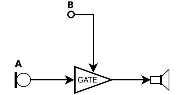
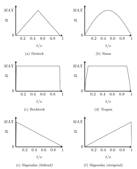
Both angles are expressed in rad and range from \(-\pi\) to \(\pi\). Figure 1 shows a virtual sound source with these two parameters.

/images/spatial/single-source.png

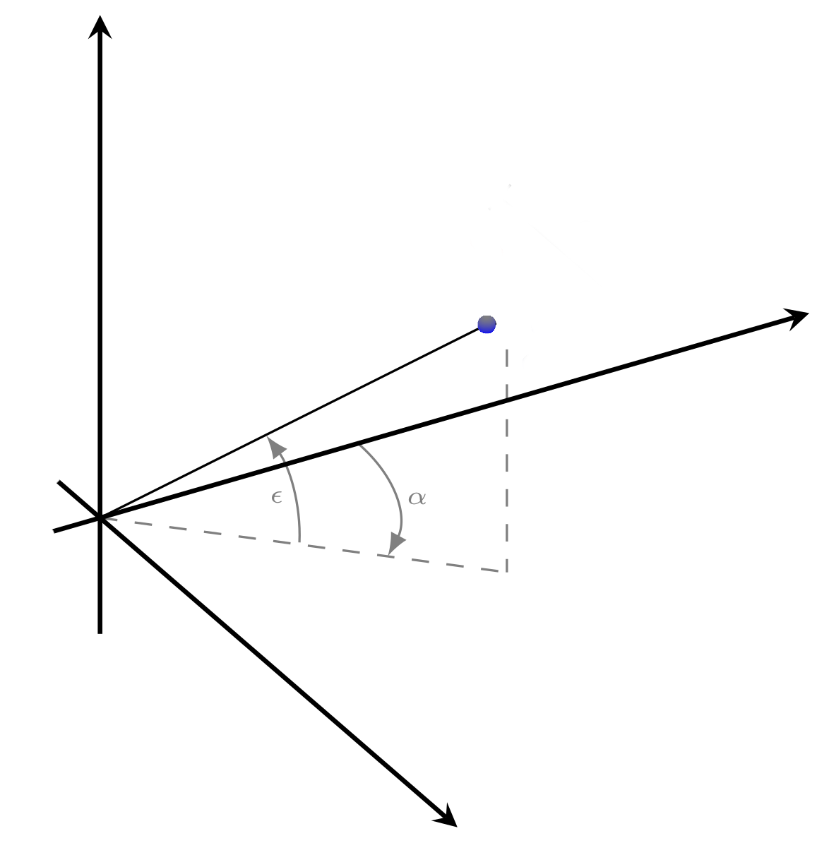
Figure 1: Virtual sound source with two angles (azimuth and elevation).

Encoding a 1st Order Source

The Ambisonics Bus

First thing to create is an audio rate bus for the encoded Ambisonics signal. The bus size depends on the Ambisonics order M, following the formula \(N = (M+1)^2\). For simplicity, this example uses first order:

s.boot;

// create the Ambisonics mix bus

~order     = 1;
~nHOA      = (pow(~order+1,2)).asInteger;
~ambi_BUS  = Bus.audio(s,~nHOA);

The channels of this bus correspond to the spherical harmonics. They encode the overall pressure and the distribution along the three basic dimensions. In the SC-HOA tools, Ambisonics channels are ordered according to the ACN convention and normalized with the N3D standard (Grond, 2017). The channels in the bus thus hold the three main axes in the following order:

Ambisonics channel ordering in the SC-HOA tools (ACN).

Spherical Harmonic Index

Channel

Description

1

W

omnidirectional

2

X

left-right

3

Z

top-bottom

4

Y

front-rear


The Encoder

The SC-HOA library includes different encoders. This example uses the HOASphericalHarmonics class. This simple encoder can set the angles of incidence (azimuth, elevation) in spherical coordinates. Angles are controlled in radians:

  • azimuth = 0 with elevation=0 is a signal straight ahead

  • azimuth =-pi/2 is hard left

  • azimuth = pi/2 is hard right

  • azimuth = pi is in the back.

  • elevation = pi/2 is on the top

  • elevation = -pi/2 is on the bottom

This example uses a sawtooth signal as mono input and calculates the four Ambisonics channels.

~encoder_A = {arg azim=0, elev=0;
      Out.ar(~ambi_BUS,HOASphericalHarmonics.coefN3D(~order,azim,elev)*Saw.ar(140));
      }.play;

The Ambisonics bus can be monitored and the angles of the source can be set, manually:

~ambi_BUS.scope;

// set parameters
~encoder_A.set(\azim,0)
~encoder_A.set(\elev,0)

The Decoder

The SC-HOA library features default binaural impulse responses, which need to be loaded first:

// load binaural IRs for the decoder
HOABinaural.loadbinauralIRs(s);

Afterwards, a first order HOABinaural decoder is fed with the encoded Ambisonics signal. It needs to be placed after the encoder node to get an audible output to the left and right channels. This output is the actual binaural signal for headphone use.

~decoder = {HOABinaural.ar(~order, In.ar(~ambi_BUS,~nHOA))}.play;
~decoder.moveAfter(~encoder_A);


Panning Multiple Sources

Working with multiple sources requires a dedicated encoder for each source. All encoded signals are subsequently routed to the same Ambisonics bus and a single decoder is used to create the binaural signal. The angles of all sources can be set, individually.

~encoder_B = {arg azim=0, elev=0;
         Out.ar(~ambi_BUS,HOASphericalHarmonics.coefN3D(~order,azim,elev)*Saw.ar(277))}.play;

~encoder_B.set(\azim,pi/4)
~encoder_B.set(\elev,1)

Exercises


References

2017

  • Florian Grond and Pierre Lecomte. Higher order ambisonics for supercollider. In Linux audio conference 2017 proceedings. 2017.
    [details] [BibTeX▼]

HaLaPhon & Luigi Nono

Principle

The HaLaPhon, developed by Hans Peter Haller at SWR in the 70s and 80s, is a device for spatialized performances of mixed music, and live electronics. The first version was a fully analog design, whereas the following ones used analog signal processing with digital control. The HaLaPhon principle is based on digitally controlled amplifiers (DCA), which are placed between a source signal and loudspeakers. It is thus a channel-based-panning paradigm. Source signals can be tape or microphones:

/images/spatial/halaphon/halaphon_GATE.png

DCA (called 'Gate') in the HaLaPhon.


Each DCA can be used with an individual characteristic curve for different applications:

/images/spatial/halaphon/halaphon_kennlinien.png

DCA: Different characteristic curves.


Quadraphonic Rotation

A simple example shows how the DCAs can be used to realize a rotation in a quadraphonic setup:

/images/spatial/halaphon/halaphon_circle.png

Circular movement with four speakers.


/images/spatial/halaphon/halaphon_4kanal.png

Quadraphonic setup with four DCAs.


Envelopes

The digital process control of the HaLaPhon generates control signals, referred to as envelopes by Haller. Envelopes are generated through LFOs with the following waveforms:

/images/spatial/halaphon/halaphon_huellkurven1.png

Circular movement with four speakers.


Envelopes for each loudspeaker gain are synchronized in the control unit, resulting in movement patterns. These can be stored on the device and triggered by the sound director or by signal analysis:

/images/spatial/halaphon/halaphon_programm1.png

Quadraphonic setup with four DCAs.


Prometeo

Haller worked with various composers at SWR. His work with Luigi Nono, especially the ambituous Prometeo, showed new ways of working with the live spatialization of mixed music. The HaLaPhon's source movements could be triggered and controlled by audio inputs, thus merging sound and space more directly.


/images/spatial/nono-111.jpg

Construction for 'Prometeo' in San Lorenzo (Venice).

/images/spatial/prometheo_movements.jpg

Sketch of spatial sound movements in 'Prometeo'.


References

2018

  • Christoph von Blumröder. Zur bedeutung der elektronik in karlheinz stockhausens œuvre / the significance of electronics in karlheinz stockhausen's work. Archiv für Musikwissenschaft, 75(3):166–178, 2018.
    [abstract▼] [details] [BibTeX▼]

2015

  • Martha Brech and Henrik von Coler. Aspects of space in Luigi Nono's Prometeo and the use of the Halaphon. In Martha Brech and Ralph Paland, editors, Compositions for Audible Space, Music and Sound Culture, pages 193–204. transctript, 2015.
    [details] [BibTeX▼]
  • Michael Gurevich. Interacting with Cage: realising classic electronic works with contemporary technologies. Organised Sound, 20:290–299, 12 2015. doi:10.1017/S1355771815000217.
    [details] [BibTeX▼]

2011

  • John Chowning. Turenas: the realization of a dream. In Proceedings of the 17th Journées d\rq Informatique Musicale. 2011.
    [details] [BibTeX▼]

2010

2008

  • Marco Böhlandt. “kontakte” – reflexionen naturwissenschaftlich-technischer innovationsprozesse in der frühen elektronischen musik karlheinz stockhausens (1952–1960). Berichte zur Wissenschaftsgeschichte, 31(3):226–248, 2008.
    [details] [BibTeX▼]
  • Jonas Braasch, Nils Peters, and Daniel Valente. A loudspeaker-based projection technique for spatial music applications using virtual microphone control. Computer Music Journal, 32:55–71, 09 2008.
    [details] [BibTeX▼]

Wait for (Audio) Hardware in systemd

Wait for (Audio) Hardware

In some cases it can be necessary to wait for a specific device, like a USB interface, before starting a service with systemd. This is the case for the JACK server in some setups.

With system.device

''systemd.device'' makes it possible to let services depend on the state of specific hardware. The following instructions work only for a static hardware setup and can fail if the hardware configuration is changed.

First: Find if systemd has a unit configuration file for the device. The following code lists all devices:

$ systemctl --all --full -t device

This will be a lot of output. Narrow down the search by grepping for the ALSA name of the device - in this case 'Track':

$ systemctl --all --full -t device | grep Track

The output looks as follows in this case:

sys-devices-pci0000:00-0000:00:14.0-usb2-2\x2d2-2\x2d2:1.0-sound-card1.device                               loaded active plugged M-Audio Fast Track

The '.device' identifier can now be used in the UNIT description's parts After and Requires:

[Unit]
Description=Jack audio server
After=sound.target sys-devices-pci0000:00-0000:00:14.0-usb2-2\x2d2-2\x2d2:1.0-sound-card1.device
Requires=sys-devices-pci0000:00-0000:00:14.0-usb2-2\x2d2-2\x2d2:1.0-sound-card1.device

Waveguide Strings in Faust

Waveguides are physical models of one-dimensional oscillators. They can be used for emulating strings, reeds and other components. A more detailed explanation is featured in the Sound Synthesis Introduction. The following example implements a string with losses, excited with a triangular function.

text


Faust Code

Load this example in the Faust online IDE for a quick start.

import("all.lib");

// use '(pm.)l2s' to calculate number of samples
// from length in meters:

segment(maxLength,length) = waveguide(nMax,n)
with{
nMax = maxLength : l2s;
n = length : l2s/2;
};


// one lowpass terminator
fc = hslider("lowpass",1000,10,10000,1);
rt = rTermination(basicBlock,*(-1) : si.smooth(1.0-2*(fc/ma.SR)));

// one gain terminator with control
gain = hslider("gain",0.99,0,1,0.01);
lt = lTermination(*(-1)* gain,basicBlock);


idString(length,pos,excite) = endChain(wg)
with{

nUp   = length*pos;

nDown = length*(1-pos);

wg = chain(lt : segment(6,nUp) : in(excite) : out : segment(6,nDown) : rt); // waveguide chain
};

length = hslider("length",1,0.1,10,0.01);
process = idString(length,0.15, button("pluck")) <: _,_;

References

2018

  • Romain Michon, Julius Smith, Chris Chafe, Ge Wang, and Matthew Wright. The faust physical modeling library: a modular playground for the digital luthier. In International Faust Conference. 2018.
    [details] [BibTeX▼]

2007

Audio Buffers

Most systems for digital signal processing and music programming process audio in chunks, which are defined by a so called buffer size. These buffer sizes are usually powers of 2, usually ranging from $16$ samples - which can be considered a small buffer size - to $2048$ samples (and more). Most applications, like DAWs and hardware interfaces allow the user to select this parameter. Technically this means that a system collects (or buffers) single samples - for example from an ADC (analog-digital-converter) - until the buffer is filled. This compensates irregularities in the speed of execution for single operations and ensures a jitter-free processing.


Latency

The choice of the buffer size $N$ is usually a trade-off between processor load and system latency. Small buffers require faster processing whereas large buffers keep the user waiting until a buffer has been filled. In combination with the sampling rate $f_s$, the buffer-dependent latency can be calculated as follows:

$$ \tau = \frac{N}{f_s} $$

Round trip latency usually considers both the input and output buffers, thus doubling the latency. For a system running at $48\ \mathrm{kHz}$ with a buffer size of $128$ samples - a typical size for a decent prosumer setup - this results in a round trip latency of $5.5\ \mathrm{ms}$. This value is low enough to allow a perceptually satisfying interaction with the system. When exceeding the $10\ \mathrm{ms}$ threshold it is likely that percussions and other timing-critical instruments experience disrupting latency.


Buffers in Programming

In higher level programming environments like PD, MAX, SuperCollider or Faust (depending on the way it is used), users usually do not need to deal with the buffer size. When programming in C or C++, most frameworks and APIs offer a processing routine which is based on the buffer size. This accounts for solutions like JUCE or the JACK API, but also when programming externals or extensions for the above mentioned higher level environments. These processing routines, also referred to as callback, are called by an interrupt once the the hardware is ready to process the next buffer.

Pulse Width Modulation: Example

Pitch:

Manual Pulse Width:

Time Domain:

Frequency Domain:

Working with Images

Getting the sprawl access point image

Download the operating system image for the sprawl access points! According to its postfix .xz the image is compressed with the XZ compression algorithm. Before writing the image to the sd card it has to be decompressed.

On Ubuntu/Debian you can install xz-utils and use unxz:

$ sudo apt-get install xz-utils
unxz sprawl_pi_image_20200628_shrinked.img.xz

On MacOS try the unarchiver. On Windows try the usual way to decompress files or download xz-utils.

Writing images on sd card

MacOS

➜  ~ diskutil list
/dev/disk0 (internal, physical):
   #:                       TYPE NAME                    SIZE       IDENTIFIER
   0:      GUID_partition_scheme                        *1.0 TB     disk0
   1:                        EFI EFI                     209.7 MB   disk0s1
   2:                 Apple_APFS Container disk1         1000.0 GB  disk0s2

/dev/disk1 (synthesized):
   #:                       TYPE NAME                    SIZE       IDENTIFIER
   0:      APFS Container Scheme -                      +1000.0 GB  disk1
                                 Physical Store disk0s2
   1:                APFS Volume OWC Aura Pro SSD - Data 520.8 GB   disk1s1
   2:                APFS Volume Preboot                 82.6 MB    disk1s2
   3:                APFS Volume Recovery                525.8 MB   disk1s3
   4:                APFS Volume VM                      2.1 GB     disk1s4
   5:                APFS Volume OWC Aura Pro SSD        11.2 GB    disk1s5

/dev/disk2 (internal, physical):
   #:                       TYPE NAME                    SIZE       IDENTIFIER
   0:     FDisk_partition_scheme                        *63.9 GB    disk2
   1:             Windows_FAT_32 boot                    268.4 MB   disk2s1
   2:                      Linux                         63.6 GB    disk2s2

disk2 seems to be the sd card with 64 GB. To access the raw device /dev/rdisk2 is used. To write to this device you have to be root (administrator). Unmount the device before using dd.

diskutil unmountDisk /dev/disk2
sudo dd if=rpi.img of=/dev/rdisk2 bs=4M

Linux

$ sudo dd if=rpi.img of=/dev/disk/by-id/
ata-PLDS_DVD-RW_DS8A8SH_S45N7592Z1ZKBE0758TK
ata-SAMSUNG_MZMPA016HMCD-000L1_S11BNEACC10413
ata-SAMSUNG_MZMPA016HMCD-000L1_S11BNEACC10413-part1
ata-SAMSUNG_MZMPA016HMCD-000L1_S11BNEACC10413-part2
ata-SAMSUNG_MZMPA016HMCD-000L1_S11BNEACC10413-part3
ata-SanDisk_SSD_PLUS_240GB_184302A00387
ata-SanDisk_SSD_PLUS_240GB_184302A00387-part1
ata-SanDisk_SSD_PLUS_240GB_184302A00387-part2
ata-SanDisk_SSD_PLUS_240GB_184302A00387-part3
ata-SanDisk_SSD_PLUS_240GB_184302A00387-part4
ata-SanDisk_SSD_PLUS_240GB_184302A00387-part5
mmc-SDC_0x000000e2
mmc-SDC_0x000000e2-part1
wwn-0x5001b448b9edd143
wwn-0x5001b448b9edd143-part1
wwn-0x5001b448b9edd143-part2
wwn-0x5001b448b9edd143-part3
wwn-0x5001b448b9edd143-part4
wwn-0x5001b448b9edd143-part5
$ sudo dd if=rpi.img of=/dev/disk/by-id/mmc-SDC_0x000000e2 bs=4M status=progress

Windows

On Windows the easiest way to write an image to a sd card is to use a dedicated application like Balena Etcher.

Wavefolding Example

The following example calculates the spectrum of a sinusoidal function, folded with a sinusoidal transfer function:

Pitch:

Pre-Gain:

Time Domain:

Frequency Domain:

Using APIs with Python

Python & APIs

With the modules requests and json it is easy to get data from APIs with Python. Using the above introduced methods for sequencing, the following example requests a response from https://www.boredapi.com/:

#!/usr/bin/env python3

import requests
import json

response = requests.get("https://www.boredapi.com/api/activity")
data     = response.json()

print(json.dumps(data, sort_keys=True, indent=4))

# print(data["activity"])