Real strings, however, introduce losses when reflecting the waves at either end.
These losses are caused be the coupling between string and body, as well as the resonant behavior of the body itself. Thus, they contribute significantly to the individual sound of an instrument.
In physical modeling, these losses can be implemented by inserting filters between the delay lines:
With an additional lowpass between the waveguides, the signal will get smoother with every iteration, resulting in a crisp onset with a sinusoidal decay. This example works with a basic moving average filter (FIR with boxcar frequency response) with a length of $N=20$.
The slow version shows the smoothing of the excitation function for both delay lines even during the first iterations:
Feedback in Faust is implemented with the ~ operator.
The left hand side of the operator declares the forward processing,
whereas the right hand side contains the processing in the feedback branch.
This example does not make sense in terms of audio processing but shows the
application of feedback.
The feedback signal is multiplied with 0.1 and simply added to the forward signal:
process=+~(_*0.1);
The related flow chart:
Feedback Example
Combined with a variable delay, the feedback operator can be used to create a simple
delay effect with adjustable delay time and feedback strength:
import("stdfaust.lib");// two parameters as horizontal slidersgain=hslider("Gain",0,0,1,0.01);delay=hslider("Delay",0,0,10000,1);// source signal is a pulsetrainsig=os.lf_imptrain(1);// the processing functionprocess=sig:+~(gain*(_,delay:@));
Partial tracking is the process of detecting single sinusoidal components in a signal and obtaining
their individual amplitude, frequency and phase trajectories.
Monophonic Partial Tracking
STFT
A short term Fourier transform segments a signal into frames of equal length.
Fundamental Frequency Estimation
YIN (de Cheveigné et al, 2002)
Swipe (Camacho, 2007)
Peak Detection
For every STFT frame, local maxima are calculated in the range of integer multiples of the fundamental frequency.
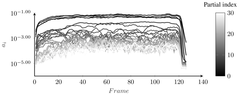
Trajectories of partial amplitudes for a violin sound.
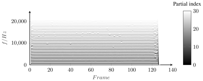
Trajectories of partial frequencies for a violin sound.
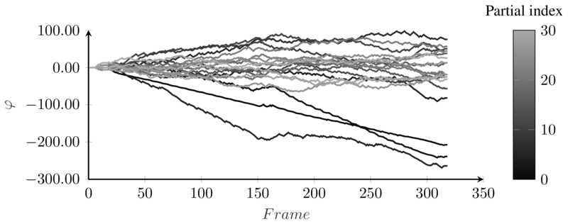
Trajectories of unwrapped partial phases for a violin sound.
classFirstClass:# Contructor, always taking the argument self + additional arguments# Is called on class instantiationdef__init__(self,a,b):self.a=aself.b=b# Methods are defined just like regular functionsdefsum(self):print(self.a+self.b)defdiff(self):print(self.a-self.b)# Create an instance of FirstClass and assigns it to the variable l:l=FirstClass(0,10)l.sum()l.diff()
Matplotlib's is a library for plotting in Python in a similar way it is handeled in Matlab.
It is usually used with pyplot - an interface for using matplotlib.
Other notable plotting libraries are Seaborn, Plotly and an API inside pandas.
The following example shows the minimum effort way of plotting with Matplotlib.
After importing pyplot and numpy, a parabola y is calculated from a set of values x.
The .plot() function takes two arguments and plots them as abcissa and ordinate, respectively:
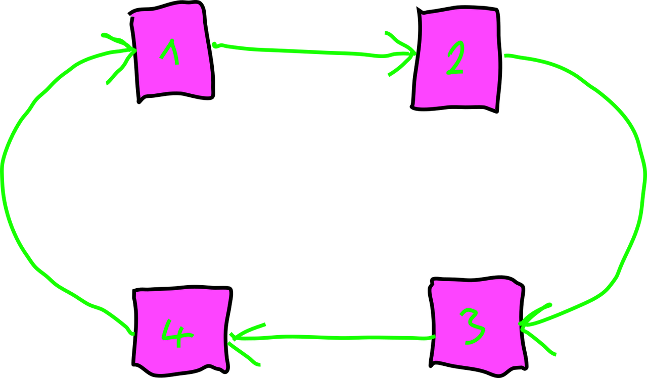
The Manual Ring is a group exercise to create a ring topology for an audio network, using JackTrip:
Four Access Points in a unidirectional circle.
In this configuration, audio signals are passed into one direction only, thus creating a closed loop. Each of the Access Points [1,2,3,4] will do additional processing before sending the signal to the next AP.
Step 1: Launch a Hub Server on each AP
The JackTrip connections for the ring are all based on the Hub-Mode - make sure to use capital Letter arguments to create Hub instances (-S and -C).
After starting a Jack server, we can launch a JackTrip Hub Server.
This process will keep running and will wait for clients to connect:
jacktrip -S
Step 2: Launch a Hub Client on each Node
Oce Hub Servers are running, Hub Clients can connect to individual servers.
Find the IP address and hostname of your left neighbor and establish a connection.
Use a single channel connection (-n 1).
Use arguments -J and -K to set the Jack client names on your own, respectively the peers machine.
Assuming we are student1 and the neighbor is student2 with the IP address 10.10.10.102, this is the command:
Using the additional arguments for the client names makes the Jack connection graph less cluttered with IP addresses.
Step 2: Boot SuperCollider and Connect
Processing of the audio signals will happen in SuperCollider. Open the scide to boot the default server by evaluating:
s.boot
In the default settings, Jack will automatically connect clients to the system's inputs and outputs. We need to remove all connections and set new ones.
The AP need no input from the system, since we will use SC to generate sound on the AP directly.
We want to pass the signal coming our of SuperCollider to our left neighbor - that is student1 and our own loudspeaker.
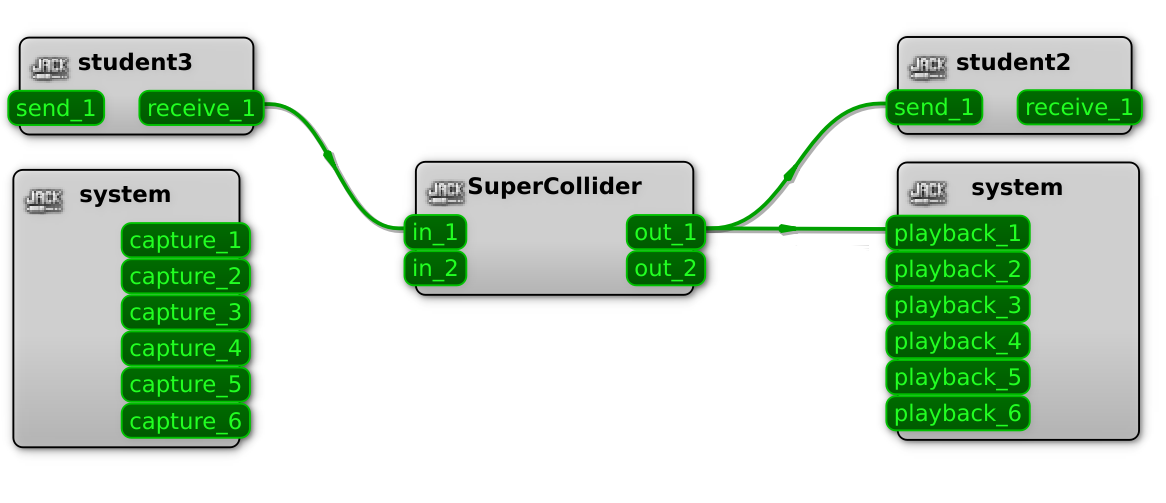
student3 sits right of student1. We want to take their signal and send it into SuperCollider for processing.
The complete Jack routing for this AP looks like this now:
Jack graph with Hub Server, Hub Client and SC server.
Step 3: Create a Processing Node on the SC Server
After all APs have performed the previous steps we have a fully connected ring. However, signals will not be passed on, since nothing is happening on the SC server.
We will create a processing node that will delay and attenuate the signal on every Access Point. This turns our ring of APs into a feedback-delay network:
With this node we are delaying the incoming signal by 0.5 seconds and passing it to the next AP with a gain of 0.95.
We can activate a server meter to see incoming and outgoing signals:
s.meter
Step 4: Send a Signal Into the Ring
With all APs connected and processing nodes in place, each AP can send a signal into the system.
The following node creates a noise burst and sends it to the next AP as well as the loudspeaker:
Force-sensing linear potentiometers (FSLPs) combine the typical force-sensing capabilities
of FSRs and in addition sense the position of the force.
This combination offers great expressive possibilities with a simple setup.
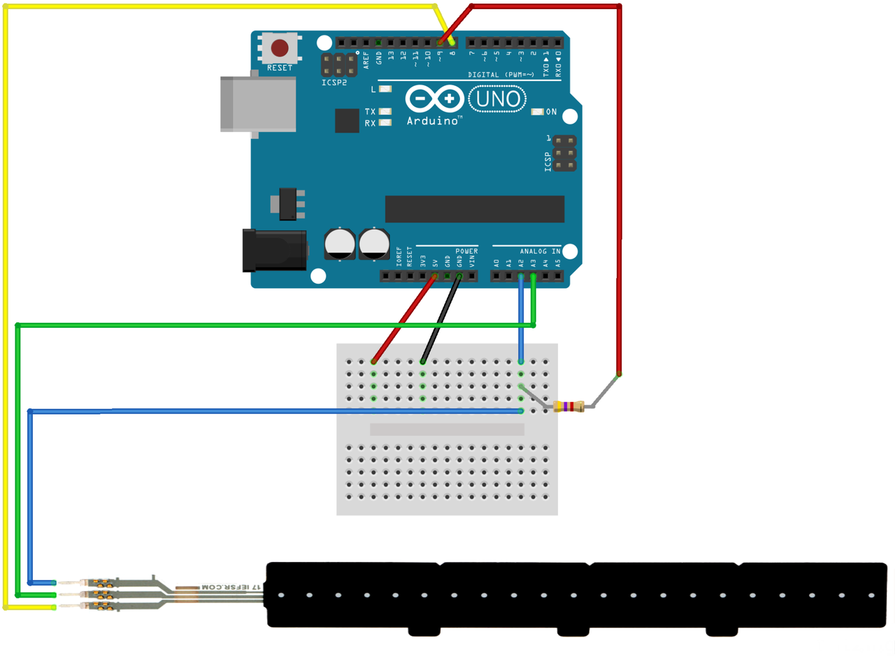
Breadboard Wiring
On the breadboard, the FSLP needs only one addition resistor of $4.7k\Omega$:
Figure: Arduino breadboard wiring.
Arduino Code
The following example is adopted from the Pololu website.
In the main loop, two dedicated functions fslpGetPressure and fslpGetPosition are used to read
force and position, respectively.
To send both values in one 'array', three individual Serial.print() commands are
used, followed by a Serial.println(). This sends a return character, allowing the
receiver to detect the end of a message block:
constintfslpSenseLine=A2;constintfslpDriveLine1=8;constintfslpDriveLine2=A3;constintfslpBotR0=9;voidsetup(){Serial.begin(9600);delay(250);}voidloop(){intpressure,position;pressure=fslpGetPressure();if(pressure==0){position=0;}else{position=fslpGetPosition();}Serial.print(pressure);Serial.print(" ");Serial.print(position);Serial.println();delay(20);}// This function follows the steps described in the FSLP// integration guide to measure the position of a force on the// sensor. The return value of this function is proportional to// the physical distance from drive line 2, and it is between// 0 and 1023. This function does not give meaningful results// if fslpGetPressure is returning 0.intfslpGetPosition(){// Step 1 - Clear the charge on the sensor.pinMode(fslpSenseLine,OUTPUT);digitalWrite(fslpSenseLine,LOW);pinMode(fslpDriveLine1,OUTPUT);digitalWrite(fslpDriveLine1,LOW);pinMode(fslpDriveLine2,OUTPUT);digitalWrite(fslpDriveLine2,LOW);pinMode(fslpBotR0,OUTPUT);digitalWrite(fslpBotR0,LOW);// Step 2 - Set up appropriate drive line voltages.digitalWrite(fslpDriveLine1,HIGH);pinMode(fslpBotR0,INPUT);pinMode(fslpSenseLine,INPUT);// Step 3 - Wait for the voltage to stabilize.delayMicroseconds(10);// Step 4 - Take the measurement.analogReset();returnanalogRead(fslpSenseLine);}// This function follows the steps described in the FSLP// integration guide to measure the pressure on the sensor.// The value returned is usually between 0 (no pressure)// and 500 (very high pressure), but could be as high as// 32736.intfslpGetPressure(){// Step 1 - Set up the appropriate drive line voltages.pinMode(fslpDriveLine1,OUTPUT);digitalWrite(fslpDriveLine1,HIGH);pinMode(fslpBotR0,OUTPUT);digitalWrite(fslpBotR0,LOW);pinMode(fslpSenseLine,INPUT);pinMode(fslpDriveLine2,INPUT);// Step 2 - Wait for the voltage to stabilize.delayMicroseconds(10);// Step 3 - Take two measurements.intv1=analogRead(fslpDriveLine2);intv2=analogRead(fslpSenseLine);// Step 4 - Calculate the pressure.// Detailed information about this formula can be found in the// FSLP Integration Guide.if(v1==v2){// Avoid dividing by zero, and return maximum reading.return32*1023;}return32*v2/(v1-v2);}
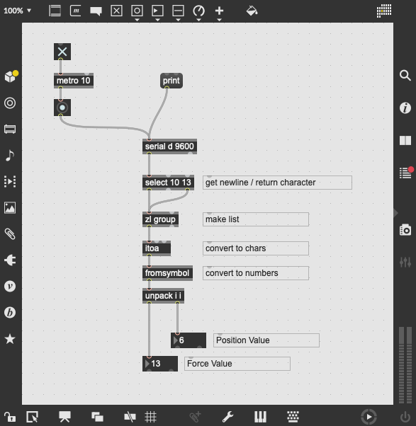
Max Patch
Extending the examples for the simple variable resistor, this patch
needs to unpack the two values sent from the Arduino.
This is accomplished with the unpack object, resulting in
two float numbers.
Without further scaling, pressure values range from 0 to 32768 ($2^{15}$),
whereas position values range from 0 to 1024 ($2^{10}$).
Figure: Max patch for receiving the two sensor values.
The history of Elektronische Musik started with
additive synthesis. In his composition Studie II,
Karlheinz Stockhausen composed timbres by superimposing
sinusoidal components.
In that era this was realized through single sine wave
oscillators, tuned to the desired frequency and recorded on tape.
The Score
Studie II is the attempt to fully compose music on a timbral level in a rigid score. Stockhausen therefor generated tables with frequencies
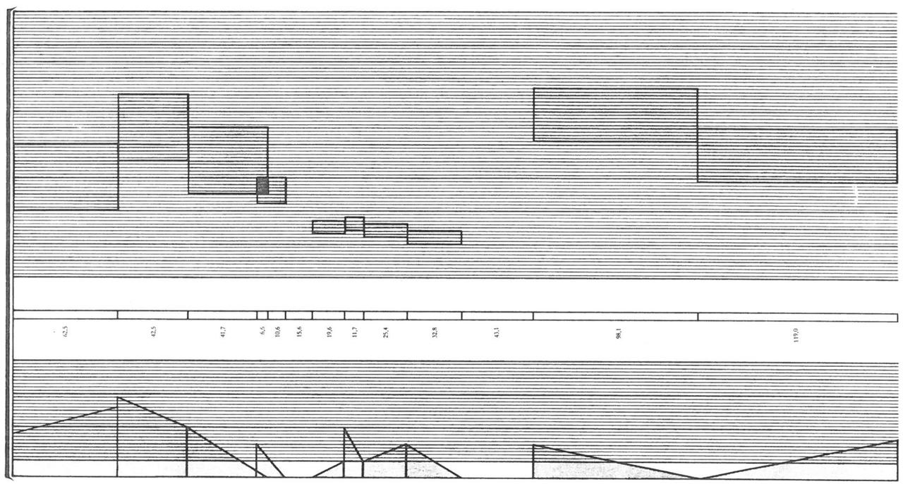
and mixed tones for creating source material. Fig.1 shows an excerpt from the timeline, which was used to arrange the material.
The timbres are recognizable through their vertical position in the upper system, whereas
the lower system represents articulation, respectively fades and amplitudes.
Fig.1: From the score of Studie II.
The Scale
Central Interval
For Studie II, Stockhausen created a frequency scale,
which not only affects the fundamental frequencies but also the overtone structure of all sounds which can be
represented by this scale.
He chose a central interval, based on the following formula:
This odd interval has 25 equally spaced pitches in 4 octaves. It is slightly higher than the semitone in the equal temperament, which has 12 equally spaced pitches in one octave:
The following buttons play both intervals starting at 443 Hz for a comparison. The difference is minute but can be detected by
trained ears:
Pitch Scale
Stockhausen used the \(\sqrt[25]{5}\) interval to create a pitch scale.
Starting from a root pitch of $100$ Hz, the scale ascends in 80 \(\sqrt[25]{5}\) steps.
However, the highest pitch value used for composing timbres lies at:
From the 81 frequencies in the pitch scale, Stockhausen creates 5 different timbres - in German Tongemische.
Each timbre is based on the \(\sqrt[25]{5}\) interval but with five different spread factors, namely 1,2,3,4 and 5.
The following table shows all five timbres for the base frequency of 100 Hz, with the spread factor in the exponent:
@article{di1998compositional,
author = "Di Scipio, Agostino",
title = "Compositional models in Xenakis's electroacoustic music",
journal = "Perspectives of New Music",
year = "1998",
pages = "201--243",
publisher = "JSTOR"
}
1870
Hermann von Helmholtz.
Die Lehre von den Tonempfindungen als physiologische Grundlage für die Theorie der Musik, 3. umgearbeitete Ausgabe.
Braunschweig: Vieweg, 1870. [details]
[BibTeX▼]
@book{vonhelmoltz1870dielehre,
author = "von Helmholtz, Hermann",
title = {Die Lehre von den Tonempfindungen als physiologische Grundlage f{\"u}r die Theorie der Musik, 3. umgearbeitete Ausgabe},
publisher = "Braunschweig: Vieweg",
year = "1870"
}
The following example uses 16 granular synths in parallel,
each being rendered as an individual virtual sound source with
azimuth and elevation in the 3rd order Ambisonics domain.
This allows the synthesis of spatially distributed sound textures,
with the possibility of linking grain properties their spatial position.
A Granular SynthDef
The granular SynthDef creates a monophonic granular stream with individual
rate, output bus and grain position.
It receives a trigger signal as argument.
// a synthdef for grains(SynthDef(\spatial_grains,{|buffer=0,trigger=0,pos=0.25,rate=1,outbus=0|varc=pos*BufDur.kr(buffer);vargrains=TGrains.ar(1,trigger,buffer,rate,c+Rand(0,0.1),0.1);Out.ar(outbus,grains);}).send;)
A Trigger Synth
The trigger synth creates 16 individual random trigger signals, which are sent to
a 16-channel audio bus.
The density of all trigger streams can be controlled via an argument.
An array of 16 granular Synths creates 16 individual grain streams, which are sent to
a 16-channel audio bus.
All Synths are kept in a dedicated group to ease the control over the signal flow.
An array of 16 3rd order decoders is created in a dedicated encoder group.
This group is added after the granular group to ensure the correct order of
the synths.
All 16 encoded signals are sent to a 16-channel audio bus.
A decoder is added after the encoder group and fed with the encoded Ambisonics
signal.
The binaural output is routed to outputs 0,1 - left and right.
// load binaural IRs for the decoderHOABinaural.loadbinauralIRs(s);(~decoder={Out.ar(0,HOABinaural.ar(3,In.ar(~ambi_BUS.index,16)));}.play;)~decoder.moveAfter(~encoder_GROUP);