OSC: Open Sound Control

Open Sound Control (OSC) is the standard for exchanging control data between audio applications in distributed systems and on local setups with multiple components. Almost any programming language and environment for computer music offers means for using OSC, usually builtin.

OSC is based on the UDP/IP protocol in a client-server paradigm. A server needs to be started for listening to incoming messages sent from a client. For bidirectional communication, each participant needs to implement both a server and a client. Servers start listening on a freely chosen port, whereas clients send their messages to an arbitrary IP address and port.

The ports 0 to 1023 are reserved for common TCP/IP applications and can thus not be used in most cases.


OSC Messages

A typical OSC message consists of a path and an arbitrary number of arguments. The following message sends a single floating point value, using the path /synthesizer/volume/:

/synthesizer/volume/ 0.5

The path can be any string with slash-separated sub-strings, as paths in an operating system. OSC receivers can sort the messages according to the path. Parameters can be integers, floats and strings. Unlike MIDI, OSC offers only the transport protocol but does not define a standard for musical parameters. Hence, the paths used for a certain software are completely arbitrary and can be defined by the developers.

First Sounds with SuperCollider

Boot a Server

Synthesis and processing happens inside an SC server. So the first thing to do when creating sound with SuperCollider is to boot a server. The ScIDE offers menu entries for doing that. However, using code for doing so increases the flexibility. In this first example we will boot the default server. It is per default associated with the global variable s:

// boot the server
s.boot;

A First Node

In the SC server, sound is generated and processed inside synth nodes. These nodes can later be manipulated, arranged and connected. A simple node can be defined inside a function curly brackets:

// play a sine wave
(
{
    // calculate a sine wave with frequency and amplitude
    var x = SinOsc.ar(1000);

    // send the signal to the output bus '0'
    Out.ar(0, x);

}.play;

)

UGens

Inside the synth node, the UGen (Unit Generator) SinOsc is used. UGens are the binary building blocks for signal processing on the server. Most UGens can be used with audio rate (.ar) or control rate (.kr).


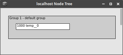
In the ScIDE, there are several ways to get information on the active nodes on the SC server. The node tree can be visualized in the server menu options or printed from sclang, by evaluating:

s.queryAllNodes

After creating just the sine wave node, the server will show the following node state:

NODE TREE Group 0
   1 group
      1001 temp__1

The GUI version of the node tree looks as follows. This representation is updated in real time, when left open:

/images/basics/sc-nodes-1.png

Note

The server itself does not know any variable names but addresses all nodes by their ID. IDs are assigned in an ascending order. The sine wave node can be accessed with the ID 1001.


Removing Nodes

Any node can be removed from a server, provided its unique ID:

s.sendMsg("/n_free",1003)

All active nodes can be removed from the server at once. This can be very handy when experiments get out of hand or a simple sine wave does not quit. It is done by pressing Shift + . or evaluating:

// free all nodes from the server
s.freeAll

Running SC Files

SuperCollider code is written in text files with the extensions .sc or .scd. On Linux and Mac systems, a complete SC file can be executed in the terminal by calling the language with the file as argument:

$ sclang sine-example.sc

The program will then run in the terminal and still launch the included GUI elements.

Using JACK Audio

The JACK API implements an audio server, allowing the connection of various software clients and hardware interfaces. In short, it turns the whole system into a digital audio workstation (DAW). It is the the standard way of working on Linux (pro) audio systems, but is also available for Mac and Windows. JACK needs a back end to connect to the actual audio hardware. On Linux systems, this is usually ALSA (Mac uses Core Audio and Windows ASIO).


Starting a JACK Server

A JACK server can be started via various graphical tools, such as QjackCtl or Carla. Many audio programs also boot a JACK server o their own, if launched. The recommended way of starting a JACK server in our case is the terminal, using the command jackd. It takes several arguments. The following line starts a server (in the background) with the ALSA interface named PCH, using a sample rate of 48kHz and a buffer size of 128 samples.

$ jackd -d alsa -d hw:PCH -r 48000 -p 128 &

Finding ALSA Devices

One way of finding the ALSA name of your interface is to type the following command:

$ aplay -l

The output shows all ALSA capable devices, their name listed after the card x:. PCH is usually the default onboard sound card:

**** List of PLAYBACK Hardware Devices ****
card 0: HDMI [HDA Intel HDMI], device 3: HDMI 0 [HDMI 0]
  Subdevices: 1/1
  Subdevice #0: subdevice #0
card 0: HDMI [HDA Intel HDMI], device 7: HDMI 1 [HDMI 1]
  Subdevices: 1/1
  Subdevice #0: subdevice #0
card 0: HDMI [HDA Intel HDMI], device 8: HDMI 2 [HDMI 2]
  Subdevices: 1/1
  Subdevice #0: subdevice #0
card 0: HDMI [HDA Intel HDMI], device 9: HDMI 3 [HDMI 3]
  Subdevices: 1/1
  Subdevice #0: subdevice #0
card 0: HDMI [HDA Intel HDMI], device 10: HDMI 4 [HDMI 4]
  Subdevices: 1/1
  Subdevice #0: subdevice #0
card 1: PCH [HDA Intel PCH], device 0: CX20751/2 Analog [CX20751/2 Analog]
  Subdevices: 1/1
  Subdevice #0: subdevice #0

Connecting JACK Clients

As almost everything, JACK connections can be modified from the terminal. All available JACK ports can be listed with the following command:

$ jack_lsp

Two ports can be connected with the following command:

$ jack_connect client1:output client2:input

Disconnecting two ports is done as follows:

$ jack_disconnect client1:output client2:input

If possible, a GUI-based tool, such as QjackCtl, can be more handy for connecting clients. It can be started via the a Desktop environment or from the command line:

$ qjackctl

/images/basics/qjackctl_connect.png

QjackCtl with hardware connections and two clients.


Storing/Restoring Connections

Several tools allow to store and restore JACK connections. Some of them work in a dynamic way, detecting spawned clients and connecting them accordingly. Others just allow a single operation for restoring connections.

aj-snapshot

The command line tool aj-snapshot is automatically installed alongside JACK. It can store and restore both JACK and ALSA connections, which can be handy when working with MIDI and is the most feature-rich and robust solution.

Once all connections are set, they can be stored to in an XML file, specified by a single argument:

aj-snapshot connections.snap

The above stored connections can be restored with the flag -r. An additional x deletes all prior connections, thus restoring the original state in the file:

aj-snapshot -xr connections.snap

The tool can also be started as a demon, looking for new clients and setting the related connections:

aj-snapshot -d connections.snap

Note

In some spatial audio projects, hardware devices and clients can have many a large number of ports. aj-snapshot does not handle that well and takes an excessive amount of time for deleting existing connections.


jmess

jmess is another command line tool, storing and restoring only JACK connections. It does not come with a demon mode but is a lot faster than aj-snapshot.


jack-matchmaker

jack matchmaker is a Python-based command line tool for dynamically restoring previously saved JACK connections.


QjackCtl Patchbay

The QjackCtl Patchbay offers a graphical solution for storing JACK and ALSA connections. Once activated, it patches new clients dynamically.

Filters in PD

Filters are an essential, sound-defining component within subtractive synthesis. Especially in analog hardware, filters of specific instruments, like the TB 303 or the Minimoog, make the individual - almost legendary - sound qualities. It thus makes sense to look for different filter implementations in software, since they can improve the overall sound a lot. PD offers a couple of builtin filters but additional externals come with more elaborate implementations.


"User-Friendly" Filters

lop~, hip~ and bp~ are the basic non-resonant filters in PD. The PD Floss Manuals on filters give a nice introduction to these builtin one-pole filters. The PD help files also come with examples. Due to the lacking resonance, these filters are not the most interesting ones, musically. They are also called "user-friendly", since they can not become unstable.

With the example one-pole-filters.pd from the repository, different characteristics of the one-pole filters can be compared, using a band-limited sawtooth as input signal. Filter cutoff and quality are controlled with control rate signals:

/images/Sound_Synthesis/subtractive/pd-one-pole-filters.png

Resonant Lowpass Filters

Additional filters can be implemented or installed with Deken. Filters and the relevant extensions can be found in the list of external filters . The iemlib, for example, features many useful resonant filters. One is the 8th order resonant lowpass vcf_lp8~. The moog~ filter object from the flatspace ggee library is another good sounding implementation, trying to emulate the famous Moog Ladder sound. The example resonant-lowpass.pd compares the sound of these filters with a square wave input. For both implementations, all parameters are controlled with audio rate signals. The slider values are thus converted to signals with the line~ object, which is basically a linear interpolation.

/images/Sound_Synthesis/subtractive/pd-resonant-lowpass.png

Exercises

Exercise I

Control the parameters of the resonant lowpass example with temporal envelopes (ADSR). Use one ADSR for the signal amplitude and one for the cutoff frequency. If the ADSR for the cutoff has a faster decay-release than the one for the amplitude, the sound fill have a sharp onset and a damped release.

Exercise II

Trigger the envelope with a metronome sequencer.

Exercise III

Create a square wave from the sawtooth and use it as input signal (http://write.flossmanuals.net/pure-data/square-waves/).

Physical Modeling: Introduction

Physical modeling emulates actual physical processes with digital means. Oscillators, resonators and acoustic impedance are modeled with buffers and filters, respectively LTI systems. Although first realized when computers had sufficient power, the foundations are much older. Hiller et al. (1971) were the first to transport the 1774 wave equation by d'Alambert to the digital domain for synthesizing sounds of plucked strings.


Early Hardware

Although physical modeling algorithms sound great, offer good means for control and enable the design of interesting instruments, they had less impact on the evolution of music genres and digital instruments. Hardware synths for physical modeling from the 1990s, like the Korg Prophecy or the Yamaha VL1 did not become a success, in the first place. With prices of about 10.000 $, they were way too expensive. There are many more practical reasons for the lack of success (Bilbao et al, 2019). But the technique also had a bad timing, trying to establish in the 1990s. Cheaper and larger memory made sampling instruments more powerful and virtual analog synthesizers sounded more attractive, followed by the second wave of analog synths.


Yamaha VL1 (1994)


Software Instruments

Today, some physical modeling software emerged for high quality piano and organ synthesis (Amazona article). Other implementations aim at strings:

  • Pianoteq Pro 6

  • Organteq Alpha

  • Strum GS 2

  • AAS Chromophone 2


Modular

Since simple physical models are nowadays easily implemented on small embedded systems, various modules exist on the market. It a modular setup, this is especially interesting, since arbitrary excitation signals can be generated and patched. These are just two examples:

/images/Sound_Synthesis/physical_modeling/mysteron.jpg
/images/Sound_Synthesis/physical_modeling/rings.jpg

Physical Models in Experimental Music

Eikasia

Unlike FM synthesis, subtractive synthesis or sampling, physical modeling does not come with genre-defining examples from popular music. However, the technique has been used a lot in the context of experimental music (Chafe, 2004). Eikasia (1999) by Hans Tutschku was realized using the IRCAM software Modalys:


S-Morphe-S

In his 2002 work S-Morphe-S, Matthew Burtner used physical models of singing bowls, excited by a saxophone:


References

2019

  • Stefan Bilbao, Charlotte Desvages, Michele Ducceschi, Brian Hamilton, Reginald Harrison-Harsley, Alberto Torin, and Craig Webb. Physical modeling, algorithms, and sound synthesis: the ness project. Computer Music Journal, 43(2-3):15–30, 2019.
    [details] [BibTeX▼]

2004

  • Chris Chafe. Case studies of physical models in music composition. In Proceedings of the 18th International Congress on Acoustics. 2004.
    [details] [BibTeX▼]

1995

  • Vesa Välimäki. Discrete-time modeling of acoustic tubes using fractional delay filters. Helsinki University of Technology, 1995.
    [details] [BibTeX▼]
  • Gijs de Bruin and Maarten van Walstijn. Physical models of wind instruments: A generalized excitation coupled with a modular tube simulation platform*. Journal of New Music Research, 24(2):148–163, 1995.
    [details] [BibTeX▼]

1993

  • Matti Karjalainen, Vesa Välimäki, and Zoltán Jánosy. Towards High-Quality Sound Synthesis of the Guitar and String Instruments. In Computer Music Association, 56–63. 1993.
    [details] [BibTeX▼]

1992

  • Julius O Smith. Physical modeling using digital waveguides. Computer music journal, 16(4):74–91, 1992.
    [details] [BibTeX▼]

1971

  • Lejaren Hiller and Pierre Ruiz. Synthesizing musical sounds by solving the wave equation for vibrating objects: part 1. Journal of the Audio Engineering Society, 19(6):462–470, 1971.
    [details] [BibTeX▼]
  • Lejaren Hiller and Pierre Ruiz. Synthesizing musical sounds by solving the wave equation for vibrating objects: part 2. Journal of the Audio Engineering Society, 19(7):542–551, 1971.
    [details] [BibTeX▼]

Concept of Subtractive Synthesis

Functional Units

Subtractive synthesis is probably the best known and most popular method of sound synthesis. The basic idea is to start with signals with rich spectral content which are then shaped afterwards by filters. Although the possibilities of subtractive synthesis are quasi-unlimited, especially when combined with other methods, the principle can be explained with three groups of functional units:

  • Generators

  • Manipulators

  • Modulators


[Fig.1] gives an overview how these functional units are arranged in a subtractive synthesizer. Modulators and generators overlap, since they are interchangeable in many aspects. This section uses the terminology from the (modular) analog domain, with Voltage Controlled Oscillators (VCO), Voltage Controlled Filters (VCF) and Voltage Controlled Amplifiers (VCA).


/images/Sound_Synthesis/subtractive/subtractive-figure0.png
Fig.1

Functional units in subtractive synthesis.


Generators

  • Oscillators (VCO)

  • Noise Generators

  • ...

Frequently used oscillators in subtractive synthesis are the basic waveforms with high frequency energy, such as the sawtooth, square wave or the triangular wave (See the section on additive synthesis). Noise generators can be used for adding non-harmonic components.

Manipulators

  • Filters (VFC)

  • Amplifiers (VCA)

  • ...

The most important manipulators are filters and amplifiers, respectively attenuators. Filters will be explained in detail in the following sections.

Modulators

  • LFO (Low Frequency Oscillators)

  • Envelopes (ADSR)

  • ...

Modulators are such units which control the parameters of generators and manipulators over time. This includes periodic modulations, such as the LFO, and envelopes, which are triggered by keyboard interaction.


A Typical Bass/Lead Patch

Like with all methods for sound synthesis, the dynamic change of timbre is an essential target for generating vivid sounds. [Fig.2] shows a more specific signal flow which is a typical subtractive synth patch for generating lead or bass sounds.

  • The signal from a VCO is manipulated by a VCF and then attenuated by a VCA.

  • The VCO has a sawtooth or square waveform.

  • The cutoff frequency of the VCF and the amplitude of the VCA are controlled with individual envelopes.

  • If ENV2 has a faster decay than ENV1, the sound will have a crisp onset and a low decay, resulting in the typical thump.


/images/Sound_Synthesis/subtractive/subtractive-figure1.png
Fig.2

Subtractive patch for bass and lead synth.

AM & Ringmodulation: Formula & Spectrum

Amplitude Modulation vs Ringmodulation

Both amplitude modulation and ringmodulation are a multiplication of two signals. The basic formula is the same for both:

$y[n] = x[n] \cdot m[n]$

However, for ringmodulation the modulation signal is symmetric:

$y[n] = \sin\left(2 \pi f_c \frac{n}{f_s}\right) \cdot \left(\sin\left[2 \pi f_m \frac{n}{f_s}\right]\right)$

Whereas for amplitude modulation, the signal ist asymetric:

$y[n] = \sin\left(2 \pi f_c \frac{n}{f_s}\right) \cdot \left( 1+ \sin\left[2 \pi f_m \frac{n}{f_s}\right]\right)$

This differnce has an influence on the resulting spectrum and on the sound, as the following examples show.

AM Spectrum

The spectrum for amplitude modulation can be calculated as follows:

$Y[k] = DFT(y[n])$

$\displaystyle Y[k] = \sum_{n=0}^{N-1} y[n] \cdot e^{-j 2 \pi k \frac{n}{N}}$

$\displaystyle = \sum_{n=0}^{N-1} \sin\left(2 \pi f_c \frac{n}{f_s}\right) \cdot \left( 1+ \sin\left[2 \pi f_m \frac{n}{f_s}\right]\right) \cdot e^{-j 2 \pi k \frac{n}{N}}$

$\displaystyle =\sum_{n=0}^{N-1} \left( \sin\left(2 \pi f_c \frac{n}{f_s}\right) + 0.5 \left( \cos\left(2 \pi (f_c - f_m)\frac{n}{f_s}\right) - \cos\left(2 \pi (f_1 + f_m)\frac{n}{f_s}\right) \right) \right) \cdot e^{-j 2 \pi k \frac{n}{N}}$

$\displaystyle= \delta[f_1] + 0.5 \delta[f_c - f_m] + 0.5 \ \delta[f_c + f_m]$

AM creates a spectrum with a peak at the carrier frequency and two peaks below and above it. Their position is defined by the difference between carrier and modulator.

Ringmod Spectrum

$\mathcal{F} [ y(t)] = \int\limits_{-\inf}^{\inf} y(t) e^{-j 2 \pi f t} \mathrm{d}t$

$= \int\limits_{-\inf}^{\inf} \left( \sin(2 \pi f_c t) \sin(2 \pi f_s t) \right) e^{-j 2 \pi f t} \mathrm{d}t$

$= \frac{1}{2 j} \int\limits_{-\inf}^{\inf} \left( (-e^{-j 2 \pi f_c t} +e^{j 2 \pi f_c t}) (-e^{-j 2 \pi f_s t} +e^{j 2 \pi f_s t}) \right) \ e^{-j 2 \pi f t} \mathrm{d}t$

$= \frac{1}{2 j} \int\limits_{-\inf}^{\inf} \left( e^{j 2 \pi (f_c+f_s) t} - e^{j 2 \pi (f_c-f_s) t} - e^{j 2 \pi (-f_c+f_s) t} + e^{j 2 \pi (-f_c-f_s) t} \right) e^{-j 2 \pi f t}$

$= \frac{1}{2 j} \left[ \delta(f_c+f_s) -\delta(f_c-f_s) - \delta(-f_c+f_s) + \delta(-f_c-f_s) \right]$

Ringmodulation creates a spectrum with
two peaks below and above the carrier frequency. Their position is defined by the difference between carrier and modulator.
The modulator is supressed, since it is symmetric.

Fourier Series: Sawtooth

Formula

The sawtooth is an asymmetric waveform with a sharp timbre. The related Fourier series is described by the following characteristics:

  • odd and even harmonics

  • alternating sign

  • slow decrease towards higher partials

\begin{equation*} X(t) = \frac{2}{\pi} \sum\limits_{k=1}^{N} (-1)^i \frac{\sin(2 \pi i f\ t)}{i} \end{equation*}

Interactive Example

Pitch (Hz):

Number of Harmonics:

Output Gain:

Time Domain:

Frequency Domain:

In contrast to the triangular wave, the interactive example shows the occurrence of ripples at the steep edges of the waveform. The higher the number of partials, the denser the ripples. This is referred to as the Gibbs phenomenon.

Faust: Compile for SuperCollider

Faust can be used to compile SuperCollider extensions. For the sine.dsp example in the introduction:

$ faust2supercollider sine.dsp

This will produce two files:

  • the class file sine.sc

  • the binary sine.so

Note that faust2supercollider depends on ruby, which you may need to install. If missing, the .sc files will be empty. There are now warnings or errors, so this can be confusing.

Both files need to be placed in the system's SuperCollider extension directory and the class library needs to be recompiled. The class name in SuperColldier is generated by Faust:

FaustSine : UGen
{
*ar { | frequency(100.0), gain(0.0) |
^this.multiNew('audio', frequency, gain)
}

*kr { | frequency(100.0), gain(0.0) |
^this.multiNew('control', frequency, gain)
}

name { ^"FaustSine" }


info { ^"Generated with Faust" }
}

The new class can be used like this:

{FaustSine.ar(100,1)}.play;

Faust: Sequential Composition

Sequential composition is used for passing signals directly from one block to another block. In Faust, this is done with the : operator. The following example illustrates this with a square wave signal, which is processed with a low pass filter:

text


The square wave has a fixed frequency of $50\ \mathrm{Hz}$. The lowpass filter has two arguments, the first being the filter order, the second the cutoff frequency, which is controlled with a horizontal slider. Both blocks are defined and subsequently connected in the process function with the : operator. The adjustable cutoff parameter is additionally smoothed with si.smoo to avoid clicks.

Load this example in the Faust online IDE for a quick start:

import("stdfaust.lib");

freq  = hslider("frequency",100, 10, 1000, 0.001);

sig  = os.square(50);
filt = fi.lowpass(5,freq);

process = sig:filt;